
How I used Python, D3 and Flask to create this interactive visualization
Almost 72 years ago, acclaimed American writer Kurt Vonnegut came up with a novel method for graphing the plot lines of stories as part of his master’s thesis in anthropology.
Although his work was ultimately rejected by the University of Chicago “because it was so simple and looked like too much fun,” according to Vonnegut, his overlooked contribution has received some renewed attention in the last few years after a group of researchers from the University of Vermont decided to use computational methods to test his hypothesis.
What they came up with were computer-generated story arcs for nearly 2,000 books in English, categorized into one of the six main storytelling arcs outlined in Vonnegut’s original thesis. These include “Rags to Riches” (rise), “Riches to Rags” (fall), “Man in a Hole” (fall then rise), “Icarus” (rise then fall), “Cinderella” (rise then fall then rise) and “Oedipus” (fall then rise then fall).
Their work deviated from Vonnegut’s in that they plotted the emotional trajectory of stories, not just their plot lines. To do so, they slid 10,000-word windows through each text to score the relative happiness of hundreds of points in the story, using a lexicon of 10,000 unique words scored on a nine-point scale of happiness, resulting in the hedonometer tool for sentiment analysis.
Using Arousal as a Proxy Measure for Action
Using a similar lexicon-based approach, I plotted the emotional arcs of more than a thousand movie scripts and used hierarchical clustering to group the most similar scripts.
However, since previous research focuses mostly on positive and negative sentiment, rather than rising and falling action, the following method differs from UVM’s approach in that it uses the NRC Valence, Arousal and Dominance Lexicon, which has scores for 20,000 English words, as a proxy measure for action or conflict in a story. Specifically, I used the arousal dimension to score words on a spectrum from “calm” or “passive” to “excited” or “active.”
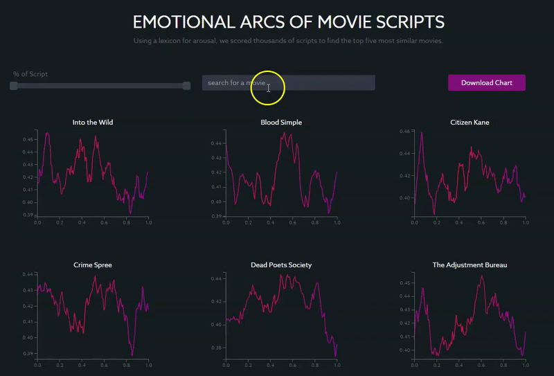
The result is an interactive visualization that can be used to search for any script already published on the Internet Movie Database to visualize its emotional story arc (for arousal) and find five of the most similar movie scripts in terms of the story’s emotional trajectory, not content.
In a search for the blockbuster “Avatar,” for example, you can see that arousal peaks towards the end of the movie, at around 90% of the length of the script, which corresponds to the point in the movie with the most tension and conflict (the final confrontation between the Na’vi and the humans to determine the fate of the planet).
Other movies with similar structures, with a clear climactic end, include “Beauty and the Beast,” “The Avengers” (2012) and “Ali.”
Here is the process I followed to arrive at these results:
Scraping Texts and Scoring Using the VAD Lexicon
Using Beautiful Soup and a revised version of Jeremy Kunn’s script, I scraped all of the movies from the Internet Movie Database, which took about 20 minutes using the following script:
import os
from urllib.parse import quote

from bs4 import BeautifulSoup
import requests

BASE_URL = 'http://www.imsdb.com'
SCRIPTS_DIR = 'scripts'


def clean_script(text):
    text = text.replace('Back to IMSDb', '')
    text = text.replace('''<b><!--
</b>if (window!= top)
top.location.href=location.href
<b>// -->
</b>
''', '')
    text = text.replace('''          Scanned by http://freemoviescripts.com
          Formatting by http://simplyscripts.home.att.net
''', '')
    return text.replace(r'\r', '')


def get_script(relative_link):
    tail = relative_link.split('/')[-1]
    print('fetching %s' % tail)
    script_front_url = BASE_URL + quote(relative_link)
    front_page_response = requests.get(script_front_url)
    front_soup = BeautifulSoup(front_page_response.text, "html.parser")

    try:
        script_link = front_soup.find_all('p', align="center")[0].a['href']
    except IndexError:
        print('%s has no script :(' % tail)
        return None, None

    if script_link.endswith('.html'):
        title = script_link.split('/')[-1].split(' Script')[0]
        script_url = BASE_URL + script_link
        script_soup = BeautifulSoup(requests.get(script_url).text, "html.parser")
        script_text = script_soup.find_all('td', {'class': "scrtext"})[0].get_text()
        script_text = clean_script(script_text)
        return title, script_text
    else:
        print('%s is a pdf :(' % tail)
        return None, None


if __name__ == "__main__":
    response = requests.get('http://www.imsdb.com/all%20scripts/')
    html = response.text

    soup = BeautifulSoup(html, "html.parser")
    paragraphs = soup.find_all('p')

    for p in paragraphs:
        relative_link = p.a['href']
        title, script = get_script(relative_link)
        if not script:
            continue

        with open(os.path.join(SCRIPTS_DIR, title.strip('.html') + '.txt'), 'w', encoding='utf-8') as outfile:
            outfile.write(script)
Then I created a new dictionary using the NRC VAD lexicon:
dict = pd.read_csv('./NRC-VAD-Lexicon-Aug2018Release/NRC-VAD-Lexicon-Aug2018Release/NRC-VAD-Lexicon.txt', sep='\t')
dict['Ranking'] = np.arange(1, len(dict)+1)
columnsTitles = ["Word","Ranking","Arousal","Valence","Dominance"]
dict = dict.reindex(columns=columnsTitles)
dict['Arousal'] = dict['Arousal'].astype(str)
newDict = dict.set_index('Word').T.to_dict('list')
And I adjusted the simple labMT usage script to calculate the arousal scores of a corpus, rather than happiness, by replacing the labMT dictionary and labMT vectors with my own:
def process():
  windowSizes = [2000]
  words = [x.lower() for x in re.findall(r"[\w\@\#\'\&\]\*\-\/\[\=\;]+",raw_text_clean,flags=re.UNICODE)]
  lines = raw_text_clean.split("\n")
  kwords = []
  klines = []
  for i in range(len(lines)):
    if lines[i][0:3] != "<b>":
      tmpwords = [x.lower() for x in re.findall(r"[\w\@\#\'\&\]\*\-\/\[\=\;]+",lines[i],flags=re.UNICODE)]
      kwords.extend(tmpwords)
      klines.extend([i for j in range(len(tmpwords))])

  for window in windowSizes:
    breaks = [klines[window/10*i] for i in range(int(floor(float(len(klines))/window*10)))]
    breaks[0] = 0
    f = open("word-vectors/"+str(window)+"/"+movie+"-breaks.csv","w")
    f.write(",".join(map(str,breaks)))
    f.close()
    chopper(kwords,labMT,labMTvector,"word-vectors/"+str(window)+"/"+movie+".csv",minSize=window//10)

    f = open("word-vectors/"+str(window)+"/"+movie+".csv","r")
    fullVec = [list(map(int,line.split(","))) for line in f]
    f.close()

    # some movies are blank
    if len(list(fullVec)) > 0:
      if len(list(fullVec[0])) > 9:
        precomputeTimeseries(fullVec,labMT,labMTvector,"timeseries/"+str(window)+"/"+movie+".csv")
    else:
      print("this movie is blank:")
      print(movie.title)
      movie.exclude = True
      movie.excludeReason = "movie blank"
Considering that movie scripts are shorter on average than books, I set the fixed window size at 1,000 words and slid it through each script to generate n arousal scores, or the number of points in the resulting time series.
Matrix Decomposition and Hierarchical Clustering
After implementing the revised version of simple labMT, which uses singular value decomposition under the hood to find a decomposition of stories onto an orthogonal basis of emotional arcs, I used linear interpolation to create word vectors of equal dimensions and used scipy’s hierarchical clustering to find and group the most similar movie scripts based on the trajectory of their emotional arcs.
from scipy.cluster.hierarchy import fcluster

import scipy.cluster.hierarchy as hac

Z = hac.linkage(df_interpolate.iloc[:,0:266], method='ward', metric='euclidean')

# k Number of clusters I'd like to extract
results = fcluster(Z, k, criterion='maxclust')
Using Ward’s method and Euclidean distance as the distance metric, I was able to minimize the variance between clusters of movie scripts to arrive at the most accurate segmentation of observations.
Using Flask API to Score and D3 to Visualize Results
Finally, I created a Flask API to output arousal scores for any movie found in the Internet Movie Database and return the five most similar scripts.
Using a function to call the API and filter the data, I visualized the resulting output using D3’s built-in d3.json() method for loading and parsing json data objects.
function updateData(){
    d3.json('https://storyplotsapp.herokuapp.com/api', {
        method:"POST",
        body: JSON.stringify({
        movie_title: ItemSelect
        }),
        headers: {"Content-type": "application/json; charset=UTF-8"}
        }).then(function(data){
            console.log(data);
        // // Prepare and clean data
        filteredData = {};
        for (var movie in data) {
            if (!data.hasOwnProperty(movie)) {
                continue;
            }
            filteredData[movie] = data[movie];
            filteredData[movie].forEach(function(d){
                d["score"] = +d["score"];
                d["percent"] = +d["percent"];
                d["cluster3"] = +d["cluster3"];
            });
            console.log(filteredData);
        }
        d3.selectAll("svg").remove();

        indexSearch = d3.keys(data).indexOf(ItemSelect);
        var indexes = [0,1,2,3,4,5]
        new_array = indexes.filter(function checkIndex(index) {
            return index !== indexSearch;
        });
        console.log(new_array);

        lineChart1 = new LineChart("#chart-area1", d3.keys(data)[indexSearch]);
        lineChart2 = new LineChart("#chart-area2", d3.keys(data)[new_array[0]]);
        lineChart3 = new LineChart("#chart-area3", d3.keys(data)[new_array[1]]);
        lineChart4 = new LineChart("#chart-area4", d3.keys(data)[new_array[2]]);
        lineChart5 = new LineChart("#chart-area5", d3.keys(data)[new_array[3]]);
        lineChart6 = new LineChart("#chart-area6", d3.keys(data)[new_array[4]]);
    })
}
You can play around with the final interactive visualization here and view all the notebooks and code here. Let me know what you think below!
