
Geometric deep learning is a very exciting new field, but its mathematics is slowly drifting into the territory of algebraic topology and theoretical physics. This is especially true for the paper “Gauge Equivariant Convolutional Networks and the Icosahedral CNN” by Cohen et. al.(https://arxiv.org/abs/1902.04615), which I want to explore in this article. The paper uses the language of gauge theory, which lies in the center of anything in physics that likes to use the words “quantum” and “field” together. It promises to give an intuitive understanding of the basics of gauge theory and I must say, it delivers and is probably the nicest introduction I have seen so far. But it still remains a difficult subject.
What I want to do here, is give a purely intuitive understanding, with no math. While I don’t follow the structure of the paper exactly, you can still open the paper side-by-side, as I will try and highlight all important terminology.
In the following I’ll assume you know how convolutional neural networks (CNN) work, but have no idea what they have to do with manifolds. So let’s go!
Manifolds
A manifold is a simple thing. Every 2-D surface you see can be considered a manifold. The surface of a sphere, the surface of a cube, all manifolds. But its not restricted to 2-D, heck, its not even restricted to things that can be imagined. A curve is a manifold. 4-D Space-time is a manifold. Its quite general and describes a space. But let’s focus on 2-D surfaces. The simplest surface is a plane, such as a computer screen. And when we do convolution with CNNs, we usually do it on these flat images.
Let’s say, we want to predict the weather with CNNs. For a single country, this is quite easy: Use the local weather data as input and keras-keras-boom, you have a trained model. What if we want to classify the weather for the entire planet? How do you fit that onto a single image? Perhaps:

But there is a problem. The left and the right edge are the same spot in reality. Further, the entire top edge corresponds to a single point, as does the lower edge. The whole thing is distorted. Ever tried flattening a ping-pong-ball? Yeah, that doesn’t go well. When we try to apply convolution, we would get strange results. Unphysical things might happen at the edges. It might predict a strong east wind on the far right of the image, but nothing on the left side of the image, even though they represent the same spot. The CNN just doesn’t understand that the earth wraps around.
Alternatively, we could create multiple overlapping maps for the earth and have a CNN that operates on those. This collection of maps is also called an atlas. Shifting the CNN over all these individual maps, making sure to continue on the next map right at the same point they overlapped on, should then enable it to understand that the earth is round. This is the basic idea behind geometric deep learning: Directly apply deep learning to surfaces or manifolds to preserve their geometric structure. However, there’s a problem. A big one.
Let’s go to Singapore!
For now, let’s forget about weather for a second and take out a compass. Let’s say you are in Singapore. Head north, past Thailand, through China, Mongolia up to the north pole. And without changing direction, keep going forward. You’ll be going through Canada, the US until you end up somewhere in Central America. Stop right there and start swimming side-ways through the Pacific, without changing direction! After a few million strokes, you should end up back in Singapore. But wait. You never changed direction, why are you looking south?
Let’s repeat that, but this time we go sideways to the left once we reach the north pole. We’ll end up near Nigera and start walking backwards, again not changing our direction. Once we’re back in Singapore, this time we are looking west? Strange… Don’t believe me? Try it out yourself, just get a compass and start swimming…
This problem is due to the curvature of the sphere and we refer to “moving around without changing direction” as parallel transport. You saw that parallel transport is very dependent on the path taken on a sphere. On the 2-D plane, however, it doesn’t matter. You can walk every path without changing direction and have the same direction once you get back. Thus, we say that the plane is parallelizable (your direction vector stays parallel once you get back), whereas the sphere is not.
You can see that this is a problem for our CNN on a sphere. If we shift our CNN in different ways over all our maps, the direction seems to change. We need to find a way to make sure that this weirdness does not affect our result! Or, at least we should know how to deal with it.
Hairy, Hairy Balls
Before we find a solution, we must introduce more math concepts. A compass needle can be viewed as a vector on a plane pointing in some direction, mostly north. This plane the needle rotates on is tangential to the earth’s surface and we’ll refer to it as the earth’s tangent space at this spot. Even though the earth is round, the tangent space is perfectly flat. It acts like a local coordinate system with north and east being its coordinate vectors. And, as we can take our compass out at any spot on earth, each spot has its own tangent space. But we could also define 40° and 130° as our coordinate vectors. North and the other directions are nothing special in this case and the choice is arbitrary.
Now, let’s choose any direction in our tangent space and follow it with a step forward. We make sure to take the shortest path (geodesic) and end up at a new point. You might call this “going forward”, but to confuse everyone, we’ll call this process the exponential map (which comes from the fact that all these tiny steps magically resemble the series expansion of the exponential function… but that’s not important now).
Let’s look at our compass needle again. The fact that the compass assigns a vector to “every” spot on earth is called a (tangent) vector field. Wind can also be seen as a vector field, as it assigns a direction to every point. I specifically put “every” in quotes, as something goes wrong with the compass needle when you stand directly on magnetic north or magnetic south. As a matter of fact, it goes wrong for every non-zero continuous vector field on a sphere. We must have poles in our magnetic field on the sphere. This phenomena is called the hairy ball theorem, as it is akin to not being able to comb a hairy ball, without creating twirls:

Vector fields don’t need to have the same dimension as the tangent space. Instead, they can have their own vector space of arbitrary dimension at each point. This is important, because we also want to be able to assign 3-D or 99-D vectors to each point on earth and not just 2-D directions. This vector space at each point of a field is also referred to as a fiber.
(A special type of field is the scalar field. It has just one dimension and temperature can be viewed as such a scalar field)
Gauge
Temperature is measured differently everywhere. Here in Germany, we use Celsius. In the US they use Fahrenheit. This choice is called a gauge. And yes, that word derives from the measuring instrument. Now, when I read a weather forecast from the US, I have to calculate what the temperature in Fahrenheit means in Celsius. We have different frames of reference. This calculation is called a gauge transformation. Note that the actual temperature didn’t change, just the value we use to understand it and the transformation is a simple linear function.
If we look at vector fields, such as wind direction, things get more complicated. To take this to the extreme, let’s pretend theres some country, Gaugeland, that doesn’t really care about north and south and has its own direction system based on star constellations or the direction a hedgehog runs when its scared. When these people describe wind, we must perform a gauge transformation to understand the direction they are talking about. Now the gauge transformation becomes a multiplication by an invertible matrix (it must go both ways obviously). This group of matrices is calledthe general linear group or GL.
For a theoretical flat earth, a choice of gauge for wind can be global. But on a sphere, we run into problems. We can’t define a single global gauge, but must instead rely on multiple gauges and maps. From our problem of parallelization on the sphere and the hairy ball theorem, we should have some intuition why this must be so.
This automatically means, that we need multiple wind maps. However, we no longer allow all of Gaugeland’s shenaniganz and demand that at least the magnitude of the vectors they use (wind speed) must be the same as ours. We only allow them to use different directions. Each gauge transformation is thus reduced to a rotation. These transformations also form a group, namely the special orthogonal group or SO, which is a subgroup of GL. We have effectively reduced the allowed transformations our gauge theory may have, by choosing a different structure group.
Back to Deep Learning
We are back to our original problem and want to perform convolution on a vector field of wind directions. Here, the wind represents the input features. Say we want to to find tornado directions as output. We can perform convolution on “small patches” to extract these output features from the wind directions. (Note: I have no idea if this makes meteorological sense… input vectors to output vectors… that’s all we need to know)
But “small patches” is a very vague description. On the 2-D plane, it is straightforward, we can just take everything that is inside some ball around the center of the patch. This also works, to some extent, on a perfect sphere. But on an arbitrary manifold? Things get tricky. Take a look at this funky manifold:
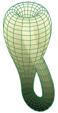
It’s called a Klein bottle and we can see that taking the raw distance between points is… problematic. We will probably never need the Klein bottle for deep learning, but we want to keep things as general as possible.
What we need is a way to only include points in convolution that are nearby on the manifold. And we do have a way to do that. Recall that the exponential map does tiny steps on our manifold to find nearby points. So let’s use that. Starting at the center, we go a step in every direction the tangent space allows us and include that point in our convolution.
All we need now is some function to do convolution with. So, we define a kernel that assigns a matrix to each poin-… wait, no, each direction of the tangent space we went with our exponential map. It’s a bit strange, but when you look at classic 2-D convolution, it actually does the same. Its just not that obvious, because its on a plane.
This matrix multiplies an input vector and produces an output vector. Here, the authors identified the first problem. This matrix is only defined for the center. But we are applying it to field vectors of nearby points, that have their own weird properties. On a plane, this isn’t a problem, but on our sphere, they are slightly different and we can’t just apply the kernel.
Let’s fix that and parallel transport the vectors at those points back to the center of our little patch. Here, we can apply our matrix, without having to worry about weird curvature problems.
Gauge Equivariance
The convolution we defined so far, seems sensible. We apply our kernels to wind data and get a nice result: tornados moving east. But somehow, we still get different results compared to Gaugeland? They predicted tornados are moving hedgehog-left?
Ahhh, yes: We need to gauge transform their result into our frame aaaand voila: They predict tornados going west... Still wrong…
What happened? We forgot to make our convolution gauge equivariant. In short, the result of the kernel must depend on the chosen gauge and transform equivariantly. If it doesn’t, we just get weird results all over that can’t be correlated or compared with one another.
But the output vector might be a different dimension or have a different interpretation than the input, how do we relate gauge transformations of the inputs to equivariant “gauge transformations” of the outputs? Well, as the structure group only acts on the inputs, the idea is to find a representation of that same group that acts on the output vectors. For example, a transformation of a 2-D input vector with a rotation group as its structure group can be represented by a 3-D output vector being rotated around a single axis. When the 2-D vector rotates, the 3-D output also rotates around a fixed axis. Generally, there can be many representations, like there could be many different rotation axis in 3-D. The point is, that it does something that represents the same action.
With the idea of representation in place, we can make convolution gauge equivariant. We just need to make sure that a gauge transformation of the input vector results in an equivariant transformation (i.e., the same transformation, but in the appropriate representation) of the output vector.
Now, with gauge equivariance, when we perform convolution on different maps, we get different results numerically, but their results agree. This is the best way we can define convolution to make sense over the entire sphere.
Icosahedron?
We basically covered Section 2 of the paper. The authors now move on to Icosahedrons, which are very similar to spheres topologically, but nicer. They are nicer in the sense that we can discretize them far more easily than the sphere.
Just like when we covered the earth with multiple maps, let’s cover the Icosahedron with 5 overlapping maps (overlap is indicated by the tiny all white triangles):
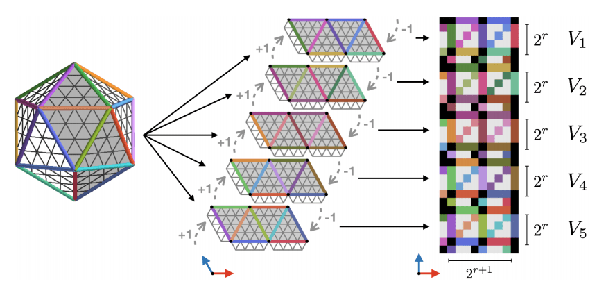
Beautiful, the maps even are the same size. No wonder they chose this manifold. We can also view it as a graph. Note that each node, i.e., each intersection, is a point on the manifold with an input feature vector (not visible in the image above). Each little triangle has 3 corners, with each corner being one of these nodes. They are what interests us.
So, let’s do convolution!
First, we need to see what our exponential map looks like. Well, on our discrete manifold, that’s easy. We just start at a node and go one step in any direction. The directions are visible in the image above as the lines connecting the nodes. So, most nodes have 6 neighbours, except those at the corners of the Icosahedron, which have 5 neighbours.
Next, we need a kernel function. But we are lazy and don’t want to reinvent the wheel. So, we’ll just use 3 x 3 filters from standard 2D convolution. These 3 x 3 filters have a center point and 8 neighbours. That’s more than we need. So, let’s just ignore the top-right and bottom-left neighbour in the 3 x 3 grid by setting them to 0 and pretend it only ever had 6 neighbours.
All that’s left is to make this thing gauge equivariant. Well, let’s look at the structure group of our Icosahedron. We already noted that we can only go in 6 different directions. If we were to describe wind on this structure, we would only have 6 different frames of reference, each rotated by 60°. This can also be formulated as having cyclic group of order 6, or C6, as its structure group.
Finally, I mentioned that our maps are overlapping. So, if we want to shift our convolutional filter over a region with overlap, we are basically using values from a different map. And what do we do with these values? We gauge transform them into the correct frame before we use them. And voila, we are doing convolution on a icosahedron.
Conclusion
In my opinion, this paper provides a fundamental result for the field of geometric deep learning. Understanding the overall idea and importance of gauge equivariance while doing convolution is the main take-away here.
I hope my non-math explanation was helpful in understanding the ideas presented in the paper. If you find this sort of thing interesting and want the hardcore math, definitely check out Nakahara’s “Geometry, Topology and Physics”.
