From: https://towardsdatascience.com/detecting-heart-arrhythmias-with-deep-learning-in-keras-with-dense-cnn-and-lstm-add337d9e41f

Let’s detect abnormal heart beats from a single ECG signal

From: https://towardsdatascience.com/detecting-heart-arrhythmias-with-deep-learning-in-keras-with-dense-cnn-and-lstm-add337d9e41f

Introduction

Recently, I was reviewing Andrew Ng’s team’s work(https://stanfordmlgroup.github.io/projects/ecg/) on heart arrhythmia detector with convolutional neural networks (CNN). I found this quite fascinating especially with the emergence of wearable products (e.g. Apple Watch and portable EKG machines) that are capable of monitoring your heart while at home. As such, I was curious how to build a machine learning algorithm that could detect abnormal heart beats. Here we will use an ECG signal (continuous electrical measurement of the heart) and train 3 neural networks to predict heart arrhythmias: dense neural network, CNN, and LSTM.

In this article, we will explore 3 lessons:

1. split the dataset on patients not on samples
2. learning curves can tell you to get more data
3. test multiple types of deep learning models

Dataset

We will use the MIH-BIH Arrythmia dataset from https://physionet.org/content/mitdb/1.0.0/. This is a dataset with 48 half-hour two-channel ECG recordings measured at 360 Hz from the 1970s. The recordings have annotations from cardiologists for each heart beat. The symbols for the annotations can be found at https://archive.physionet.org/physiobank/annotations.shtml

Project Definition

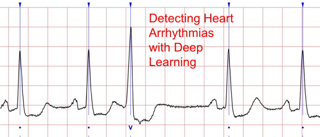
Predict if a heart beat from a ECG signal has an arrhythmia for each 6 second window centered on the peak of the heart beat.

To simplify the problem, we will assume that a QRS detector is capable of automatically identifying the peak of each heart beat. We will ignore any non-beat annotations and any heart beats in the first or last 3 seconds of the recording due to reduced data. We will use a window of 6 seconds so we can compare the current beat to beats just before and after. This decision was based after talking to a physician who said it is easier to identify if you have something to compare it to.

Data Preparation

Let’s get started by making a list of all the patients in the data_path.

Here we will use a pypi package wfdb for loading the ecg and annotations.

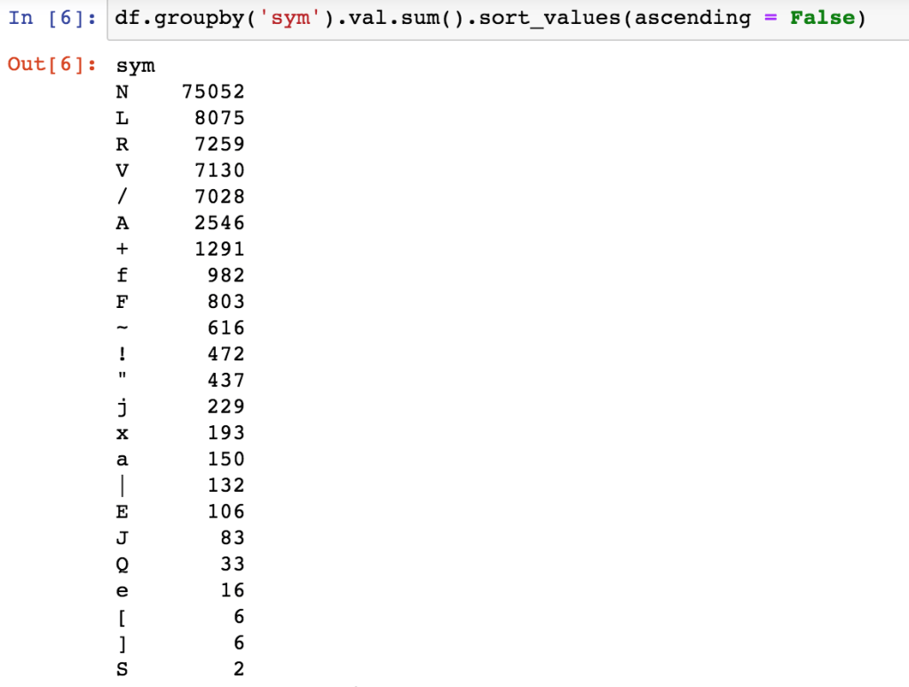
Let’s load all the annotations and see the distribution of heart beat types across all files.

We can make a list of the non-beat and abnormal beats now:

We can group by category and see the distribution in this dataset:

Looks like around 30% in this dataset are abnormal. If this was a real project, it would be good to check the literature. I imagine this is higher than normal given this is a dataset about arrhythmias!

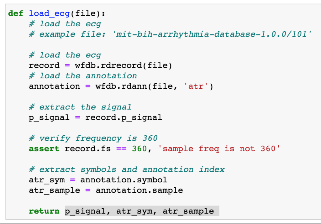
Let’s write a function for loading a single patient’s signals and annotations. Note the annotation values are the indices of the signal array.

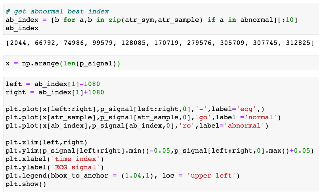
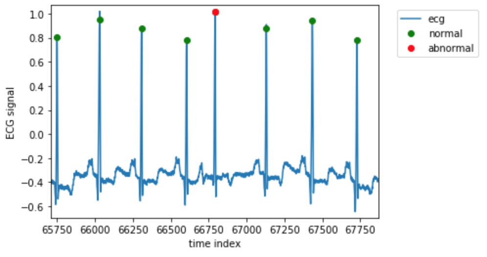
Let’s check out what abnormal beats are in a patient’s ecg:

We can plot the signal around one of the abnormal beats with:

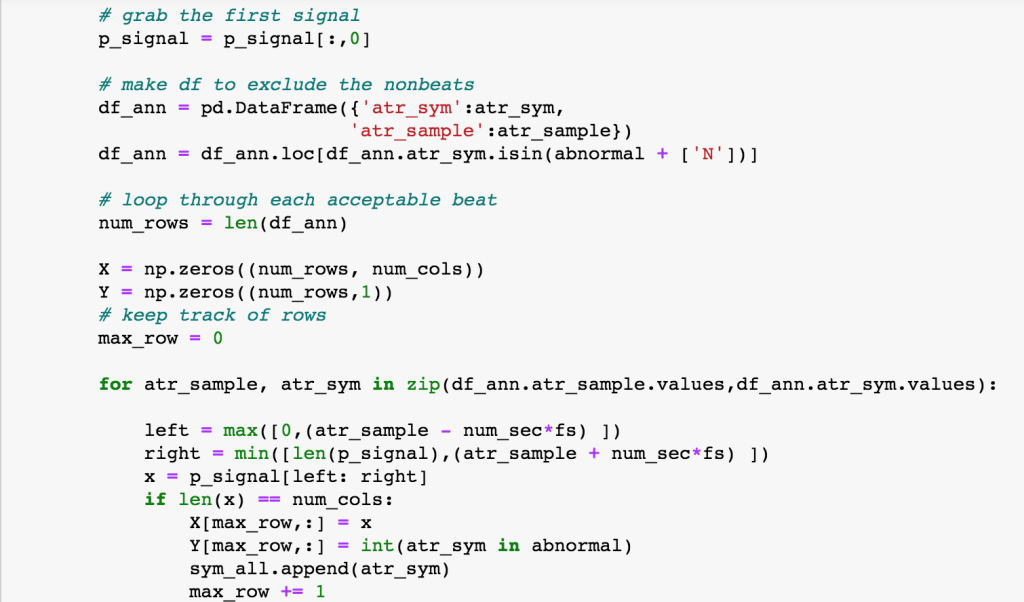
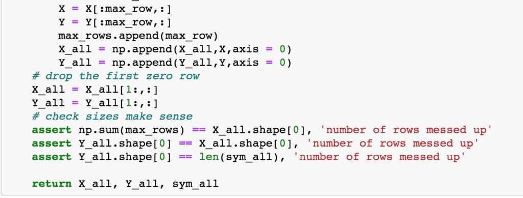
Make a dataset

Let’s make a dataset that is centered on beats with +- 3 seconds before and after [apologies for broken screenshots]

Lesson 1: split on patients not on samples

Let’s start by processing all of our patients.

Imagine we naively just decided to randomly split our data by samples into a train and validation set.

Now we are ready to build our first dense NN. We will do this in Keras for simplicity. If you would like to see the equations for dense NN and another sample project see my other post here which is a deep learning follow-up on a diabetes readmission project I wrote about here.

We can build some functions for metrics reporting. For more discussion of data science classification metrics see my prior post here.

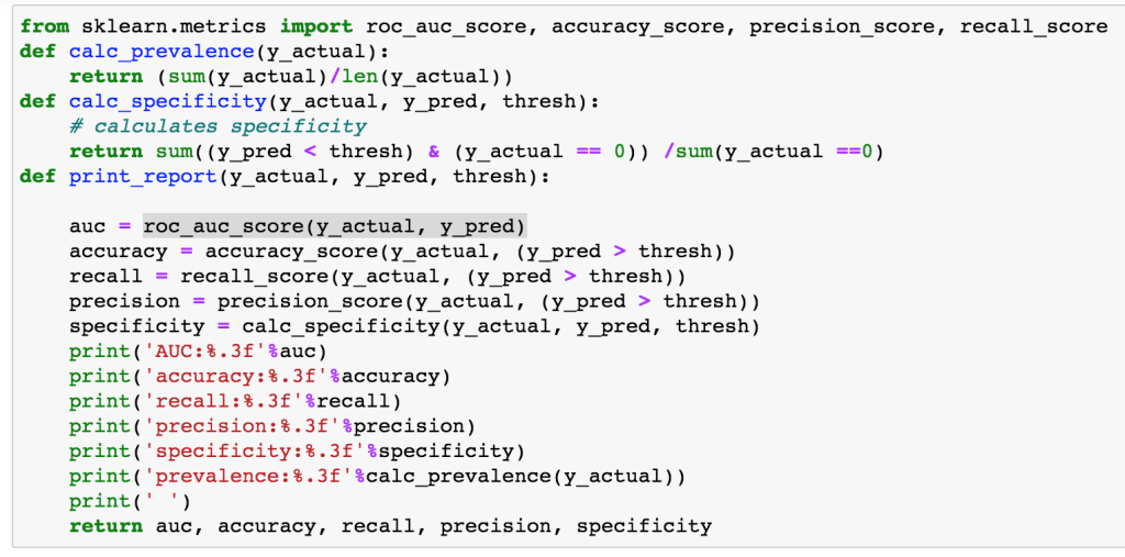
We can get the predictions from the Keras model with predict_proba

For simplicity, let’s set our threshold at the prevalence of the abnormal beats and calculate our report:

Amazing! Not that hard! But wait, will this work on new patients? Perhaps not if each patient has a unique heart signature. Technically the same patient can show up in both the training and validation sets. This means that we may have accidentally leaked information across the datasets. We can test this idea by splitting on patients instead of samples.

And train a new dense model:

As you can see the validation AUC went down by a lot, confirming we had data leakage before. Lesson learned: split on patients not on samples!

Lesson 2: learning curve can tells us we should get more data!

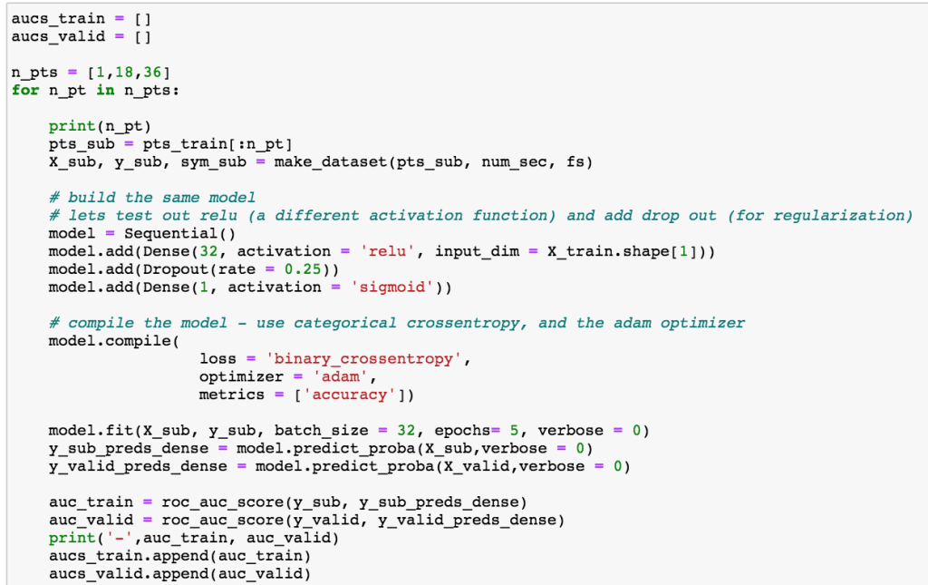
Given the overfitting between training and validation. Let’s make a simple learning curve to see if we should go collect more data.

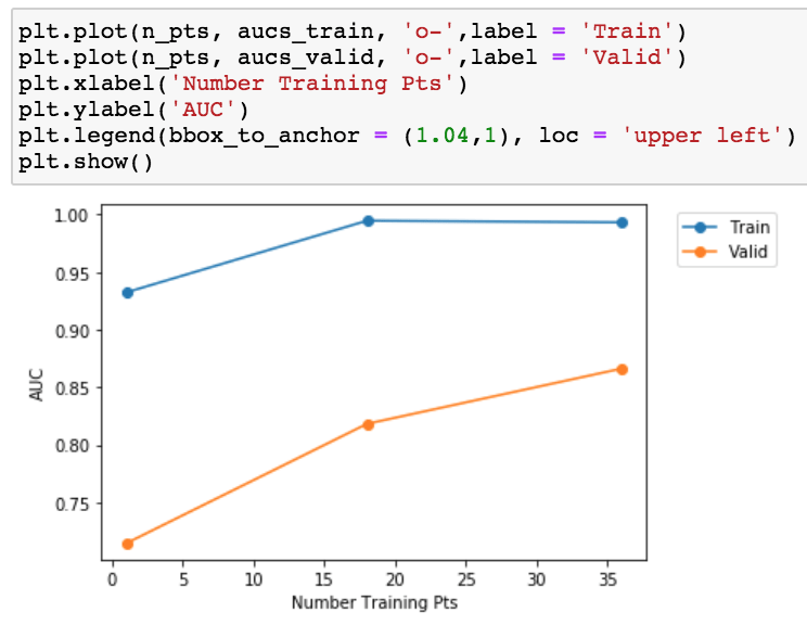
Lesson learned: more data appears to help in this project!

I suspect Andrew Ng’s team came to the same conclusion since they took the time to annotate 64,121 ECG records from 29,163 patients which is 2 orders of magnitude more than any other public dataset (see https://stanfordmlgroup.github.io/projects/ecg/).

Lesson 3: test multiple types of deep learning models

CNN

Let’s start by making a CNN. Here we will use a 1 dimensional CNN (as opposed to the 2D CNN for images).

A CNN is a special type of deep learning algorithm which uses a set of filters and the convolution operator to reduce the number of parameters. This algorithm sparked the state-of-the-art techniques for image classification. Essentially, the way this works for 1D CNN is to take a filter (kernel) of size kernel_size starting with the first time stamp. The convolution operator takes the filter and multiplies each element against the first kernel_size time steps. These products are then summed for the first cell in the next layer of the neural network. The filter then moves over by stride time steps and repeats. The default stride in Keras is 1, which we will use. In image classification, most people use padding which allows you pick up some features on the edges of the image by adding ‘extra’ cells, we will use the default padding which is 0. The output of the convolution is then multiplied by a set of weights W and added to a bias b and then passed through a non-linear activation function as in dense neural network. You can then repeat this with addition CNN layers if desired. Here we will use Dropout which is a technique for reducing overfitting by randomly removing some nodes.

For Keras’ CNN model, we need to reshape our data just a bit

Here we will be a one layer CNN with drop out

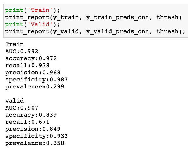
The performance seems to be higher with CNN than dense NN.

RNN: LSTM

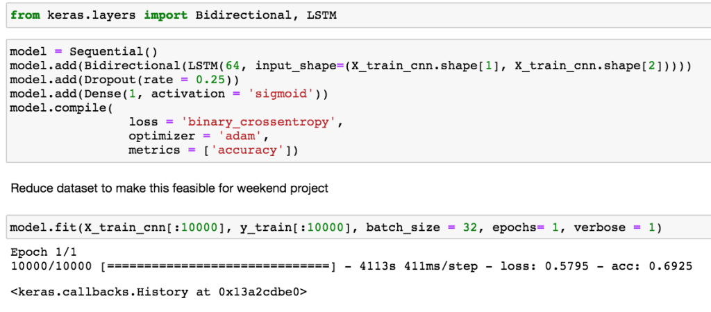
Since this data signal is time-series, it is natural to test a recurrent neural network (RNN). Here we will test a bidirectional long short-term memory (LSTM). Unlike in dense NN and CNN, RNN have loops in the network to keep a memory of what has happened in the past. This allows the network to pass information from early time steps to later time steps that usually would be lost in other types of networks. Essentially there is an extra term for this memory state in the calculation before passing through a non-linear activation function. Here we use the bidirectional information so information can be past in both direction (left to right and right to left). This will help us pick up information about the normal heart beats to the left and right of the center heart beat.

As can be seen below, this took a long time to train. To make this into a weekend project, I reduced the training set to 10,000 samples. For a real project I would increase the number of epochs and use all the samples.

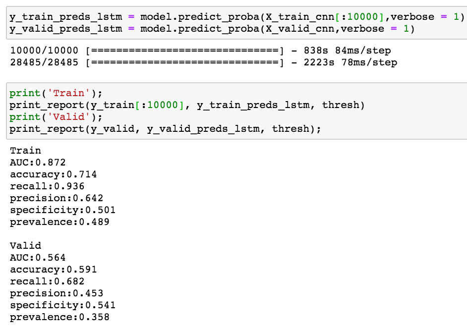
Seems like the model needs regularization (i.e. drop out) from additional epochs.

Final ROC Curve

Here’s the final ROC curves for these 3 models

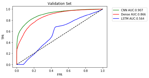
Given more time, it would be good to try to optimize the hyperparameters and see if we could get Dense or CNN even higher.

Limitations

Since this is just a weekend project, there are a few limitations:

• did not optimize the hyperparameters or number of layers
• did not collect additional data as suggested with learning curve
• did not explore literature of arrhythmia prevalence to see if this dataset is representative of the general population (probably not)

Thanks for reading!