From: https://towardsdatascience.com/noise-its-not-always-annoying-1bd5f0f240f

One of the first concepts you learn when you begin to study neural networks is the meaning of overfitting and underfitting. Sometimes, it is a challenge to train a model that generalizes your data perfectly, especially when you have a small dataset because:

• When you train a neural network with small datasets, the network generally memorizes the training dataset instead of learning general features of our data. For this reason, the model will perform well on the training set and poor on new data (for instance: the test dataset)
• A small dataset provides a poor description of our problem and thus, it may result in a difficult problem to learn.

To acquire more data is a very expensive and arduous task. However, sometimes you can apply some techniques (regularization methods) to obtain a better performance of your model.

In this article, we are focusing on the use of noise as a regularizing method in a neural network. This technique not only reduces overfitting, but it can also lead to faster optimization of our model and better overall performance.

You can find the entire code in my GitHub! 🙂

Goals

The objectives of this article are the following:

• Generate synthetic data using sklearn
• Regularization Methods
• Train a basic Neural Network as a baseline (MLP)
• Use noise as regularization method — input layer
• Use noise as regularization method — hidden layer
• Use noise as regularization method — input and hidden layer
• Grid Search to find the values for the best performance of the model

Regularization Methods

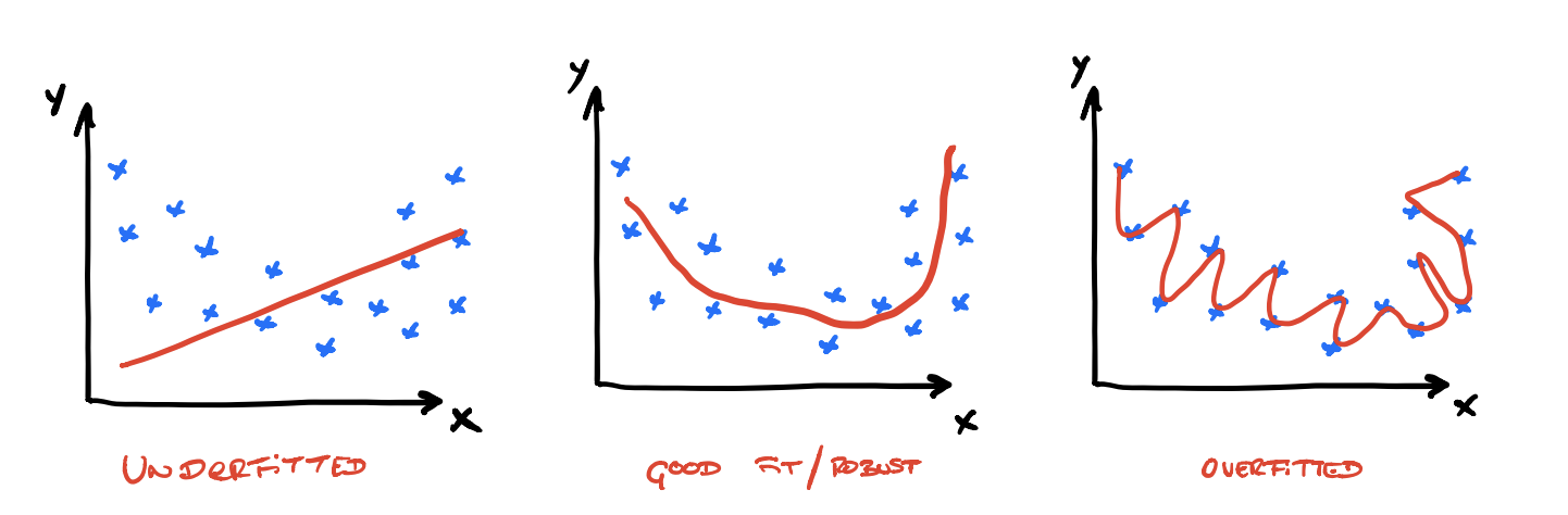
It is a challenge to train a machine learning model that will perform well on previously unseen inputs, not just those on which our model was trained. This feature is called generalization, performs well on unobserved inputs. There are some methods like train-test split or cross-validation to measure how well generalize our model.

We can classify the performance of the model in 3 cases:

• The model performs poorly on the training dataset and new data — Underfit Model.
• The model performs well on the training dataset and poorly on unseen data — Overfit Model.
• The model learns our training dataset and performs well on unseen data, it is capable to generalize — Good Fit Model

It is more likely to face overfitting models in our problems thus, it is important to monitor the performance during training to detect if it has overfitting. It is common to plot the evolution of accuracy and loss during the training to detect usual patterns.

Regularization is to modify our learning algorithm to reduce its generalization error but not its training error. The most common regularization methods in neural networks are:

• Dropout: Turn on some neuron in each iteration with probability p.
• Early Stopping: Provide guidance as to how many iterations can be run before the model begins to overfit.
• Weight Constraint: Scales weights to a pre-defined threshold.
• Noise: Introduce stochastic noise into training process.

These methods are popular in neural networks and most of them have been proven to reduce overfitting. However, the effect of noise on deep learning models has never been systematically studied, nor is the underlying reason for the improved accuracy. One hypothesis of the above observation is that relaxing consistency introduces stochastic noise into training process. This implicitly mitigates the overfitting of the model and generalizes the model better to classify test data.

Generating data using Sklearn

We want to understand the effect of using noise as a regularization method in a neural network with overfitting and we have decided to use a binary classification problem to explain this. Therefore we are going to generate a binary dataset applying sklearn, specifically make_circles which generates 2 two-dimensional concentric circles. The parameters are:

• n_samples=100 (The total number of points generated)
• noise=0.09 (Standard deviation of Gaussian noise added to the data)
• param_random=24 (Pass an int for reproducible output across multiple function calls)

# Define Parameters
n_samples = 100
param_noise = 0.1
param_random = 1

# Create Data
X_train, y_train = make_circles(n_samples=n_samples, 
                                noise=param_noise, 
                                random_state=param_random)

# Plot data
# We group the data
df = DataFrame(dict(X=X_train[:,0], Y=X_train[:,1], label=y_train))
colors = {0:'tomato', 1:'palegreen'}
fig, ax = plt.subplots(figsize=(15, 8))
grouped = df.groupby('label')

# For each group, we add it
for key, group in grouped:
    group.plot(ax=ax, kind='scatter', x='X', y='Y', s=20, label='label ' + str(key), color=colors[key])
plt.grid(alpha=0.2)
plt.show()

Generate and plot data our data

We need to evaluate the performance of our network to see if we have overfitting and thus, we need to split our data to generate another dataset x_test for testing. We have split our data into train_set (30%) and test_set (70%).

As we need to force overfitting, we have chosen a small size (30%) for our train set because we want to create a neural network that doesn’t generalize our data and has a higher error rate on the test dataset.

# Percentage for test
test_perc = 0.7

X_train, X_test, y_train, y_test = train_test_split(X_train, y_train, 
                                                    test_size=test_perc, 
                                                    random_state=42)

print("Shape of X_train: ", X_train.shape)
print("Shape of y_train: ", y_train.shape)
print("")
print("Shape of X_test: ", X_test.shape)
print("Shape of y_test: ", y_test.shape)

# We define a dataframe to group our data into 2 classes
df = DataFrame(dict(X=X_train[:,0], Y=X_train[:,1], label=y_train))
# Define color for each label
colors = {0:'tomato', 1:'palegreen'}
fig, ax = plt.subplots(figsize=(15, 8))
grouped = df.groupby('label')

# For each group, we plot it
for key, group in grouped:
    group.plot(ax=ax, kind='scatter', x='X', y='Y', s=20, label='label ' + str(key), color=colors[key])

plt.scatter(X_test[:,0], X_test[:, 1], s=10, c='black', alpha=0.6, marker='o', label='Test')
plt.grid(alpha=0.2)
plt.legend()

plt.show()

Split and plot our train and test data

We can plot the distribution of X_train and X_test:

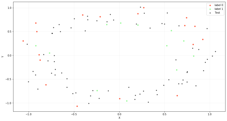
We have selected this type of data, called circle data, because these classes are not linearly separable (we can not split our data using a line). For this reason, we need a neural network to address this nonlinear problem.

As we need to find overfitting in our model to study the effect of the noise as a regularizing method, we have only generated 100 samples. This is a small size sample to train a neural network and it enables us to overfit the training.

First Step: Basic Neural Network — MLP

To study how noise influences our training, we have trained a basic Neural Network as a baseline. We have defined a Multilayer Perceptron (MLP) to address our binary classification problem.

The first layer is a hidden layer that uses 400 nodes and the relu activation function. In the output layer, we have used a sigmoid because we want to predict class values of 0 or 1. We use binary_crossentropy as loss (proper for binary classifications) and adam as optimizer.

We train the neural network for 5000 epochs and we use X_test and y_test as validation_data.

# Create model
model_basic = Sequential()
model_basic.add(Dense(400, input_dim = X_train.shape[1], activation='relu'))
model_basic.add(Dense(1, activation='sigmoid'))
model_basic.compile(loss='binary_crossentropy', optimizer='adam', metrics=['accuracy'])

model_basic.summary()

# Train model
hist_basic = model_basic.fit(X_train, y_train, 
                             validation_data=(X_test, y_test),
                             epochs=5000, 
                             verbose=0)

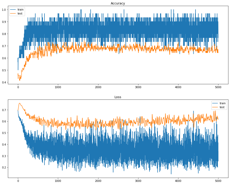
Basic Neural Network as Baseline

We have plotted a graph to represent the accuracy and loss on train and test set. It can be observed that our neural network has overfitting because this graph has the expected shape of an overfit model, test accuracy increases to a point and then begins to decrease again. At the same time, loss is divergent.

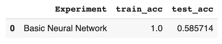
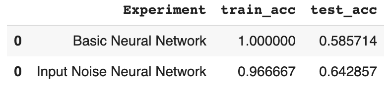
We can observe that the accuracy for the train set is about train_acc=1 and for the test set is about test_acc=0.5857. It shows better performance on the training set than in the test dataset; this can be a sign for overfitting.

Now, we are going to add noise using the Gaussian Noise Layer from Keras and compare the results. This layer applies additive zero-centered Gaussian noise, which is useful to mitigate overfitting. Gaussian Noise (GS) is a natural choice as a corruption process for real-valued inputs.

This regularization layer is only active at training time.

But what is Gaussian Noise?

Gaussian Noise is statistical noise having a Probability Density Function (PDF) equal to that of the normal distribution. It is also known as the Gaussian Distribution. The probability density function 𝑝 of a Gaussian random variable 𝑧 is given by:

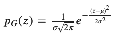
where 𝑧 represents the grey level, 𝜇 the mean value and 𝜎 the standard deviation. To sum up, the values that the noise can take on are Gaussian-distributed.

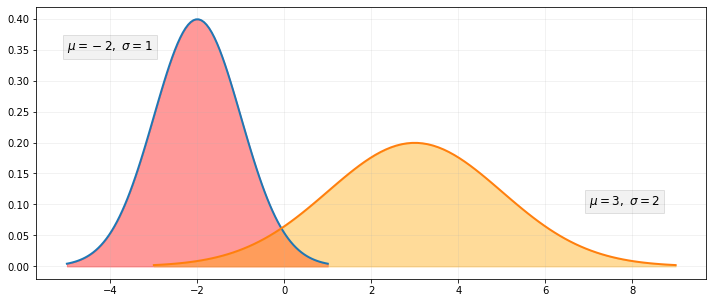
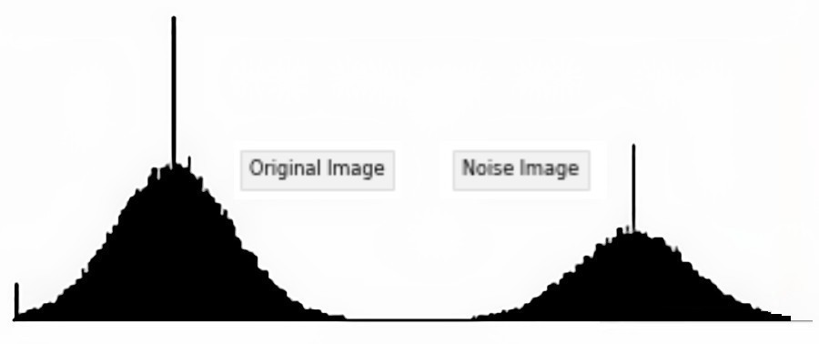
To understand the meaning of Gaussian Noise, imagine that we have an image and we have plotted 2 Probability Density Functions. If we observe the red PDF: the mean value of the noise will be -2. So, on average, 2 would be subtracted from all pixels of the image. However, if we observe the orange PDF, the mean value is 3. So on average, 3 would be added to all pixels. For instance, if we take this image and we apply Gaussian Noise:

We can check the histogram for each image to appreciate the effect of applying Gaussian Noise:

Although we have explained the Gaussian Noise with images, the method of applying Gaussian Noise as regularization methods in Keras applies the same theory.

Adding noise increases the size of our training dataset. When we are training a neural network, random noise is added to each training sample and this is a form of data augmentation. Furthermore, when we use noise, we are increasing the randomness of our data and the model is less capable to learn from training samples since they are changing each iteration. Consequently, the neural network learns more general features and has lower generalization errors.

When we apply noise, we are creating new samples in the vicinity of the training samples and thus, the distribution of the input data is smoothed. This allows the neural network to learn from our data much more easily.

Input Layer Noise in Neural Network

We will add a Gaussian Noise layer as the input layer and we are going to analyze if this helps to improve generalization performance. When we add noise we are creating more samples and making the data distribution smoother.

# Create model
model_noise_in = Sequential()
# GaussianLayer with standard deviation of 0.1
model_noise_in.add(GaussianNoise(0.1, input_shape=(2,)))
model_noise_in.add(Dense(400, activation='relu'))
model_noise_in.add(Dense(1, activation='sigmoid'))
model_noise_in.compile(loss='binary_crossentropy', optimizer='adam', metrics=['accuracy'])

model_noise_in.summary()

# Train model
hist_noise_in = model_noise_in.fit(X_train, y_train, 
                                   validation_data=(X_test, y_test),
                                   epochs=5000, verbose=0)

Neural Network with Input Layer Noise

It can be seen on the line graph that noise causes the accuracy and loss of the model to jump around due to the points with noise that we have introduced in the training and that conflict with the points of the training data set. We have used std=0.1 as input noise and which might be a little bit high.

With the use of noise as a regularization method in the input layer, we have decreased the overfitting in our model, furthermore, we have improved the test_accuracy=0.642.

Hidden Layer Noise in Neural Network

Now, we are going to try to create a Hidden Layer with Gaussian Noise. This has to be done before the activation function is applied. We will use a standard deviation of 0.1, again, chosen arbitrarily.

# Create model
model_noise_hid = Sequential()
# GaussianLayer with standard deviation of 0.1
model_noise_hid.add(Dense(400, input_dim = X_train.shape[1]))
model_noise_hid.add(GaussianNoise(0.1))
model_noise_hid.add(Activation('relu'))
model_noise_hid.add(Dense(1, activation='sigmoid'))
model_noise_hid.compile(loss='binary_crossentropy', optimizer='adam', metrics=['accuracy'])

model_noise_hid.summary()

# Train model
hist_noise_hid = model_noise_hid.fit(X_train, y_train,
                                   validation_data=(X_test, y_test),
                                   epochs=5000, verbose=0)

Neural Network with Hidden Layer Noise

In this case, it can be seen that train_accuracy remains constant, although we have managed to increase the test_accuracy=0.671. It seems that adding noise to our model allows improving the training of the neural network and is useful to mitigate overfitting.

Input + Hidden Layer Noise in Neural Network with

We have combined the 2 previous examples to study the performance of our model by adding an input layer noise and a hidden layer noise at the same time. We will use a standard deviation of 0.1, again, chosen arbitrarily.

# Create model
model_noise_in_hid = Sequential()
# GaussianLayer with standard deviation of 0.1
model_noise_in_hid.add(GaussianNoise(0.1, input_shape=(2,)))
model_noise_in_hid.add(Dense(400, activation='relu'))
model_noise_in_hid.add(GaussianNoise(0.1))
model_noise_in_hid.add(Activation('relu'))
model_noise_in_hid.add(Dense(1, activation='sigmoid'))
model_noise_in_hid.compile(loss='binary_crossentropy', optimizer='adam', metrics=['accuracy'])

model_noise_in_hid.summary()

# Train model
hist_noise_in_hid = model_noise_in_hid.fit(X_train, y_train,
                                           validation_data=(X_test, y_test),
                                           epochs=5000, verbose=0)

Neural Network with Input + Hidden Layer Noise

Once again, it can be seen that with the use of noise as input_layer and hidden_layer, at the same time, we have reduced the overfitting in our model. Additionally, it has increased the test_accuracy=0.6857 and it seems that Gaussian Noise as a regularization method allows the model to better generalize our data.

Applying noise, we are creating new samples in the vicinity of the training samples and thus, the distribution of the input data is smoothed.

Grid Search — Noise Layer

We are going to develop a grid search to find out the exact amount of noise and the nodes in the hidden layer that allow us to get the best performing model.

We will use the Neural Network with a Hidden Layer Noise as an example for the grid search. We need to create a function with the model to search for the best value for noise.

def create_model(nodes, noise_amount):

  # Create model
  model_noise_hid = Sequential()
  # GaussianLayer with standard deviation of 0.01
  model_noise_hid.add(Dense(nodes, input_dim = X_train.shape[1]))
  model_noise_hid.add(GaussianNoise(noise_amount))
  model_noise_hid.add(Activation('relu'))
  model_noise_hid.add(Dense(1, activation='sigmoid'))
  model_noise_hid.compile(loss='binary_crossentropy', optimizer='adam', metrics=['accuracy'])
  return model_noise_hid

Grid Search — Hidden Layer Noise

We have created a dictionary called grid_values that contains the range of values for each parameter of the model. Finally, we insert our model create_model() in the wrapper called KerasClassifier which implements the Scikit-Learn classifier interface.

from sklearn.model_selection import GridSearchCV
from keras.wrappers.scikit_learn import KerasClassifier

# Grid values
grid_values = {'noise_amount':[0.001, 0.01, 0.1, 0.2, 0.7, 1],
               'nodes': [50, 100, 300, 500]}

model = KerasClassifier(build_fn=create_model, epochs=5000, verbose=0, )

# Run GridSearch - It takes time
grid_model_hidden_acc = GridSearchCV(model, param_grid = grid_values)
grid_model_hidden_acc.fit(X_train, y_train)

# Plot Results
print("Best: %f using %s" % (grid_model_hidden_acc.best_score_, grid_model_hidden_acc.best_params_))
means = grid_model_hidden_acc.cv_results_['mean_test_score']
stds = grid_model_hidden_acc.cv_results_['std_test_score']
params = grid_model_hidden_acc.cv_results_['params']
for mean, stdev, param in zip(means, stds, params):
    print("%f (%f) with: %r" % (mean, stdev, param))

Calculate GridSearch

Best: 0.833333 using {'nodes': 300, 'noise_amount': 0.001} 0.766667 (0.133333) 
with: {'nodes': 50, 'noise_amount': 0.001} 0.766667 (0.133333) 
with: {'nodes': 50, 'noise_amount': 0.01} 0.766667 (0.133333) 
with: {'nodes': 50, 'noise_amount': 0.1} 0.766667 (0.081650) 
with: {'nodes': 50, 'noise_amount': 0.2} 0.700000 (0.066667) 
with: {'nodes': 50, 'noise_amount': 0.7} 0.633333 (0.124722) 
with: {'nodes': 50, 'noise_amount': 1} 0.800000 (0.163299) 
with: {'nodes': 100, 'noise_amount': 0.001} 0.800000 (0.163299) 
with: {'nodes': 100, 'noise_amount': 0.01} 0.766667 (0.133333) 
with: {'nodes': 100, 'noise_amount': 0.1} 0.800000 (0.124722) 
with: {'nodes': 100, 'noise_amount': 0.2} 0.766667 (0.169967) 
with: {'nodes': 100, 'noise_amount': 0.7} 0.666667 (0.105409) 
with: {'nodes': 100, 'noise_amount': 1} 0.833333 (0.149071) 
with: {'nodes': 300, 'noise_amount': 0.001} 0.800000 (0.163299) 
with: {'nodes': 300, 'noise_amount': 0.01} 0.766667 (0.133333) 
with: {'nodes': 300, 'noise_amount': 0.1} 0.833333 (0.105409) 
with: {'nodes': 300, 'noise_amount': 0.2} 0.666667 (0.105409) 
with: {'nodes': 300, 'noise_amount': 0.7} 0.633333 (0.124722) 
with: {'nodes': 300, 'noise_amount': 1} 0.800000 (0.163299) 
with: {'nodes': 500, 'noise_amount': 0.001} 0.800000 (0.163299) 
with: {'nodes': 500, 'noise_amount': 0.01} 0.800000 (0.124722) 
with: {'nodes': 500, 'noise_amount': 0.1} 0.833333 (0.105409) 
with: {'nodes': 500, 'noise_amount': 0.2} 0.600000 (0.133333) 
with: {'nodes': 500, 'noise_amount': 0.7} 0.600000 (0.133333) 
with: {'nodes': 500, 'noise_amount': 1}

We can see that the best results were achieved with a network with 300 neurons in the hidden layer and with noise_amount=0.001 with an accuracy of about 83%.

Future Experiments

We can improve this experiment of adding noise as regularization method with the next ideas:

• Add more layers with noise to study his effect.
• Repeat the same experiments with a deeper neural network.
• Study the effect of noise as a regularization method in a model without overfitting.
• Try to add noise to activations and weights.