

Ifyou’ve ever taken an intro finance or investment theory class, then you’ve probably come across the idea of Modern Portfolio Theory or MPT. The Nobel Prize winning idea is that we have a collection of assets which have different returns, risks and correlations with each other, and we find an optimal weighing of these assets such that the overall returns are maximized whie the variance of the returns is minimized. This idea seems quite obvious in retrospect but was revolutionary when it came out in the early 1950s.
My long and somewhat painful involvement in cryptocurrency trading has revealed that portfolio type strategies involving a basket of different cryptocurrencies do indeed tend to give reasonable returns while mitigating losses when there is a market downturn. So in this article, we will investigate a deep learning based approach to portfolio optimization and compare our models against some bench mark strategies.
Links to my other articles:
- Deep Kernels and Gaussian Processes
- Custom Loss Functions in TensorFlow
- Prediction and Inference with Boosted Trees
- Softmax classification
- Climate analysis
Introduction
The mathematical form of the return of the portfolio is a weighted average of the expected returns of each asset Rᵢ we are invested in:
The standard deviation or risk for the portfolio P return is derived here. Framed as a deep learning problem, we want to find the weights w that maximize the portfolio return P, where the weights w come from somewhere in a deep neural network (not to be confused with the weights θ of the network itself, we want to extract some outputs from the neural net and use that to weigh the portfolio).
Correlation of Assets
In an ideal world, asset prices would only go up monotonically, but in real life, especially with cryptocurrencies, there is a tremendous amount of volatility. Thus the choice of assets in the portfolio is important. Intuitively, we want to pick a basket of assets which are sufficiently different enough from each other, so that when one asset goes down, hopefully another asset goes up. In classical portfolio selection, various factors such as the price timeseries cross-correlation and perhaps other factors such as trade volume and other derived statistics may be combined to form a multidimensional similarity metric. However, my experience with cryptos has shown that the correlation between different coins can be nonlinear and is most definitely high dimensional. Thus we employ deep learning to give us a clustering of cryptos such that similarity between them can be calculated.
The method we will use to pick coins for our portfolio is from this paper: https://www.groundai.com/project/deep-convolutional-autoencoder-for-cryptocurrency-market-analysis/1 where the author trained a deep ConvNet autoencoder on price timeseries and a few other derived observables such as trade volume and high/low ratios.
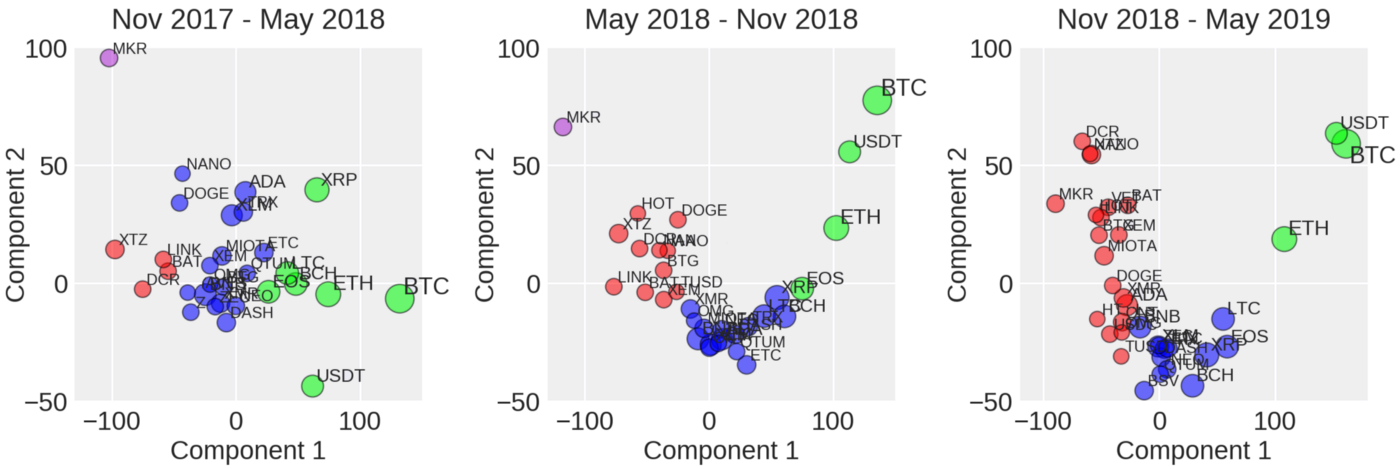
They extracted the latent tensor representation and applied PCA, and then K-means clustering to compute the clusterings. Using the clustering in the Nov 2018-May 2019 subplot, we’ll pick some randomly from each cluster and a few others not listed in the plot. Thus the coins are: ‘ETH’, ‘BTC’, ‘XMR’, ‘BCH’, ‘ADA’, ‘BAT’, ‘BNB’, ‘XTZ’.
The Model
https://github.com/hhl60492/wot2
We will borrow loosely the architecture of the encoder portion of the autoencoder model in the above paper, since that seemed to work well for the author.
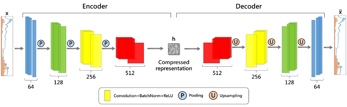
Our encoder model consists of 12 feature maps or 2D Conv layers organized into groups of 4 with batch normalization after the 2nd group. A summary of a model example is below:
Model: "model"
__________________________________________________________________________________________________
Layer (type)                    Output Shape         Param #     Connected to
==================================================================================================
input (InputLayer)              [(None, 10, 24, 1)]  0
__________________________________________________________________________________________________
conv2d (Conv2D)                 (None, 10, 24, 256)  512         input[0][0]
__________________________________________________________________________________________________
conv2d_1 (Conv2D)               (None, 10, 24, 256)  512         input[0][0]
__________________________________________________________________________________________________
conv2d_2 (Conv2D)               (None, 10, 24, 256)  512         input[0][0]
__________________________________________________________________________________________________
conv2d_3 (Conv2D)               (None, 9, 23, 128)   131200      conv2d[0][0]
__________________________________________________________________________________________________
conv2d_4 (Conv2D)               (None, 9, 23, 128)   131200      conv2d_1[0][0]
__________________________________________________________________________________________________
conv2d_5 (Conv2D)               (None, 9, 23, 128)   131200      conv2d_2[0][0]
__________________________________________________________________________________________________
batch_normalization (BatchNorma (None, 9, 23, 128)   512         conv2d_3[0][0]
__________________________________________________________________________________________________
batch_normalization_1 (BatchNor (None, 9, 23, 128)   512         conv2d_4[0][0]
__________________________________________________________________________________________________
batch_normalization_2 (BatchNor (None, 9, 23, 128)   512         conv2d_5[0][0]
__________________________________________________________________________________________________
conv2d_6 (Conv2D)               (None, 6, 20, 64)    131136      batch_normalization[0][0]
__________________________________________________________________________________________________
conv2d_7 (Conv2D)               (None, 6, 20, 64)    131136      batch_normalization_1[0][0]
__________________________________________________________________________________________________
conv2d_8 (Conv2D)               (None, 6, 20, 64)    131136      batch_normalization_2[0][0]
__________________________________________________________________________________________________
conv2d_9 (Conv2D)               (None, 1, 15, 16)    36880       conv2d_6[0][0]
__________________________________________________________________________________________________
conv2d_10 (Conv2D)              (None, 1, 15, 16)    36880       conv2d_7[0][0]
__________________________________________________________________________________________________
conv2d_11 (Conv2D)              (None, 1, 15, 16)    36880       conv2d_8[0][0]
__________________________________________________________________________________________________
flatten (Flatten)               (None, 240)          0           conv2d_9[0][0]
__________________________________________________________________________________________________
flatten_1 (Flatten)             (None, 240)          0           conv2d_10[0][0]
__________________________________________________________________________________________________
flatten_2 (Flatten)             (None, 240)          0           conv2d_11[0][0]
__________________________________________________________________________________________________
concatenate (Concatenate)       (None, 720)          0           flatten[0][0]
                                                                 flatten_1[0][0]
                                                                 flatten_2[0][0]
__________________________________________________________________________________________________
dropout (Dropout)               (None, 720)          0           concatenate[0][0]
__________________________________________________________________________________________________
output (Dense)                  (None, 8)            5768        dropout[0][0]
==================================================================================================
Total params: 906,488
Trainable params: 905,720
Non-trainable params: 768
The features we will be using are daily average (average of high, low, open and close) returns of the coins, daily volume and high/low ratios for a 10 day window, so we’ll have a 10 x (3 x number of coins) matrix of inputs for each window.
We will also need to code up a custom loss function to realize the combined objective of maximizing profit and minimizing risk. Since the default behavior of the Tensorflow/Keras (Tensorflow 2.0 is pretty much Keras now) optimizier is to minimize the loss, and we want to maximize the profit we’ll have to be a bit creative in our loss construction… duality under convexity is a beautiful thing. We will use a softmax dense layer of dimension equal to the number of coins to return the weights for the portfolio, and the weights will fall nicely in the range of sum(w) = 1, w in [0,1] so that a more qualified software engineer can code up the logic to make the actual trades/portfolio balancing.
Thus to maximize the profit while minimizing the risk of the portfolio, we’ll add a portfolio risk term to the overall loss.
We put the expected portfolio returns under a reciprocal function 1/x and add the risk term, since the default behavior of the Tensorflow optimizer is to minimize the loss.
Implementation Considerations
In light of the new and exciting TF2.0 release, I was prepared to eat my words on how convoluted it is to do custom loss functions in Keras, however it seems the ‘new’ Keras in TF 2.0 still has some issues when you attempt to put a wrapper function capable of accepting tensors as arguments around your custom loss(y_pred, y_true). It seems Tensorflow does not like taking symbolic tensors from the wrapper and spits out an error. Thus I had to put the benchmark returns as a supervised target set Y and feed it to a non-wrapper enclosed custom loss, and then everything worked out OK.
That and of course always be careful with tensor shapes.
Results
The model was trained on a single batch of the previous 500 days worth of features of the basket of assets ‘XMR’, ‘BTC’, ‘BNB’, ‘ETH’, ‘XTZ’, ‘BCH’, ‘BAT’, ‘ADA’ in that order, for 100 epochs. Some of the returned portfolio weights for the coins in the order above are:
Avg Portfolio Return (daily): 1.00120008
Avg Portfolio Risk: 0.0120014967
[0.0816616565 0.0387833901 0.1092159 0.0531964786 0.0161306579 0.618883371 0.0585224256 0.0236059185]
Compared to the benchmark values of buying and hold equal amounts of all the coins:
Overall avg return (daily): 1.0000168991159741 Overall avg risk: 0.016754081194341616
And the benchmark for individual coins:
Benchmarks, avg daily returns : avg risk
XMR.csv : 0.998491787841728 : 0.01315563029370615
BTC.csv : 1.0005725089666324 : 0.011714545830308617
BNB.csv : 1.0013448780337977 : 0.015309324427086771
ETH.csv : 0.9993215887141582 : 0.014900867160970225
XTZ.csv : 1.0013259364520484 : 0.019505261426199745
BCH.csv : 0.9993002310368153 : 0.024584067652101974
BAT.csv : 1.0009946692688383 : 0.015916325404062133
ADA.csv : 0.9987835926137753 : 0.015203108293710868
We see that the portfolio has a higher daily return by almost 71x (7100%) and the risk is lower by 28%. It’s interesting to see the portfolio weights heavily favoring Bitcoin Cash (BCH), whereas the benchmark average daily return for BCH over the previous 500 days is negative (i.e less than 1).
Of course, I’d take these results with a grain of salt and please do not construe this article and the model presented herein as investment advice in any way, shape or form. The model is a work in progress and I appreciate any feedback, insight and/or invitation for collaborative development.
The main weakness of supervised machine models in predicting the future is that they assume the future is informed by the past. To some extent cryptocurrencies exhibit this behavior (thus momentum based technical trading can be applied to some effect), but at the same time they are especially vulnerable to jumps and shocks from hype, speculation, FOMO and unforeseen events such as scandals, political upheavals, climate change, etc.
Of course, we have to mention that ‘buying and holding’ or HODLing single cryptos such as bitcoin can net a much larger return over time, but this is one of the riskiest strategies. After all, it’s a bet based on a wish and a prayer, and who knows if the Racoon Flu breaks out in the near future and devastates the global cryptocurrency market.

Some things to add for the future would be validation on holdout and online learning on new data that comes in. As always, hope you enjoyed this article, and please do be careful when trading cryptos.
