How Data Augmentation Improves your CNN performance? — An Experiment in PyTorch and Torchvision

From: https://medium.com/swlh/how-data-augmentation-improves-your-cnn-performance-an-experiment-in-pytorch-and-torchvision-e5fb36d038fb

Simple ways to boost your network performance

In simple terms, Data Augmentation is simply creating fake data. You use the data in the existing train set to create variations of it. This does two things —

1. Increases the size of your training set
2. Regularizes your network

The book Deep Learningdefines regularization as any method that modifies the learning algorithm in a way that is intended to reduce the generalization error but not the training error. In this article, we talk about one of the many methods to regularize a network — data augmentation. Specifically in images.

We use CIFAR-10, a standard dataset used for benchmarking network performance. We use is a ResNet like CNN architecture. PyTorch provides pre-trained ResNet on the ImageNet dataset (224 by 224 pixels). Since CIFAR-10 has 32 by 32 pixels images, we implement our ResNet from scratch. We will discuss the model, the dataset, augmentation approaches, results and finally the code. You may conveniently skip any part you’re not interested in.

---

The Dataset — CIFAR-10

CIFAR (Canadian Institute For Advanced Research) has prepared a dataset of 10 classes — Airplane, Automobile, Cat, Deer, Dog, Frog, Horse, Ship, Truck and Bird. The images are 32*32 pixels in size. The training set consists of 50000 images, with 5000 of each class. The test set consists of 10000 images with 1000 for each class. In our experiment, we use the train set, augment it and then calculate accuracy and loss on the validation (or test) set.

---

Model — ResNet (Residual Networks)

Modern Computer Vision applications heavily use established architectures like VGG, ResNet, Inception, etc. These models have produced good results on a wide range of Computer Vision tasks. As mentioned previously, PyTorch provides these models which are trained on the Imagenet classification dataset. For CIFAR-10, we have built our own ResNet like architecture.

Residual Blocks
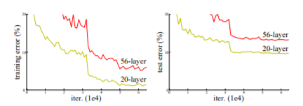
The authors of ResNet built this model to solve an important problem in training deep neural nets — Very deep neural nets are hard to train. There’s a misconception that stacking more layers improves the performance of a network. It was found that over numerous epochs, a 56-layer network gave higher train and test error rate than a 20-layer network on the CIFAR-10 dataset (Fig. 1). The authors argue that such a poor performance is not due to vanishing/exploding gradients since they have been resolved by adding normalization (references — [9, 23, 13, 37] from the paper). The reason is that deeper networks are hard to optimize.

Introducing residual blocks is a novel way to make the training of a deeper model easier. Consider two consecutive layers as shown in the figure below.

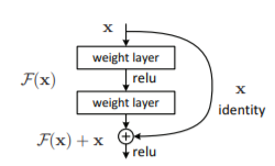
The input is x and the output is a mapping H(x). Normally, the network tries to learn the mapping H. Consider another mapping F such that

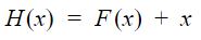
Authors of ResNet hypothesize that it is easier to learn the residual function F. The convolution operation parameters are chosen such that the dimensions of x, F(x) and H(x) in order for the addition to make sense.

---

Data Augmentation — Methods

Broadly, data augmentation in images involves changing the orientation of images, selecting a part of an image, randomly or otherwise. We discuss a few transforms here. However, a complete list of transforms can be found here.

Random Horizontal and Random Vertical Flip
To flip the image horizontally or vertically with a given probability p.

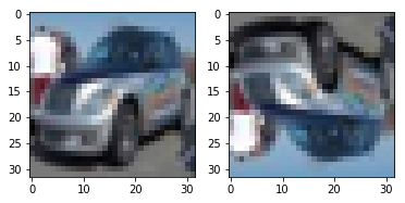
Random Crop with Padding
We pad the image with a pixel value with a defined width and the crop a desired size image from the padded image. For example, for a 32*32 image, if we pad it by 4 pixels on each side, we have a 40*40 image. We then select a random 32*32 crop from it.

Standardizing the image
The intention here is to shift the mean each pixel position to zero and variance as one.

---

Experiment and Results

Training Details —

1. Hardware — NVIDIA 1060 6 GB GPU
2. Batch Size — 128
3. Learning Rate — 0.001, weight decay — 0.0001
4. Optimizer — Adam
5. Loss — Cross-Entropy
6. Epochs/Iterations — 15

Results —

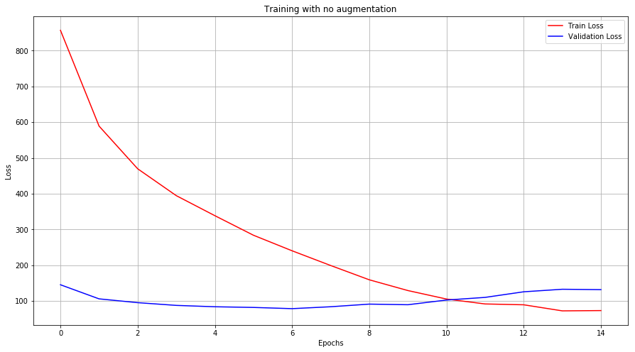
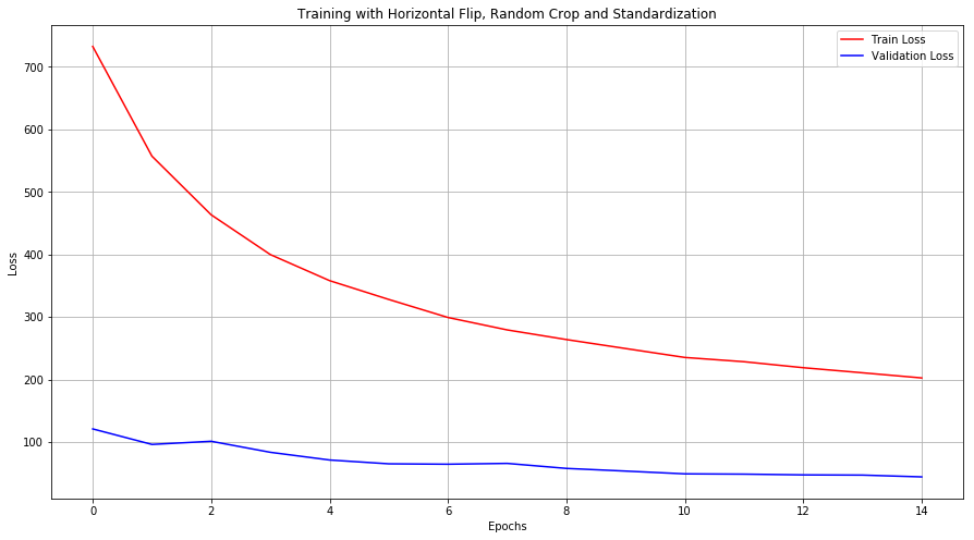
Train and Validation Loss across epochs —

Accuracies across epochs —

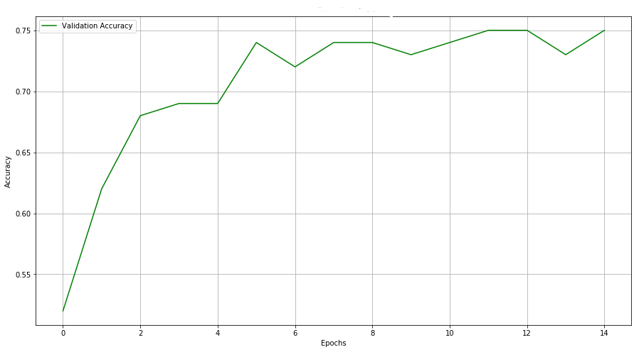
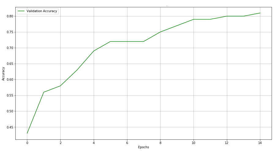
As you can see, simply augmenting the data improved our results by 6%. Moreover, it took 15 epochs to reach 76% accuracy for a dataset without augmentation. When augmented, our model reached that level of accuracy within 8 epochs.

Without augmentation, our model overfits. This is indicated by the increasing validation loss. When augmented, the model tends to not overfit within the given number of epochs.

---

Code

Finally, the code! Follow this repository —DhruvilKarani/ResNet-AugmentationPermalink Dismiss GitHub is home to over 40 million developers working together to host and review code, manage…github.com

Step 0 — Set up the model (you may skip this and use the one in the repository)

import numpy as np
import torch
import torch.nn as nn
import torchvision
from torchvision.datasets import CIFAR10
from torch.autograd import Variable
import sys
import os
import matplotlib.pyplot as plt
import seaborn as sns
from collections import Counter
import randomclass _Block(nn.Module):
    def __init__(self, kernel_dim, n_filters, in_channels, stride, padding):
        super(_Block, self).__init__()
        self._layer_one = nn.Conv2d(in_channels=in_channels, out_channels=n_filters, 
                                  kernel_size=kernel_dim, stride=stride[0], padding=padding, bias=False)
        self._layer_two = nn.Conv2d(in_channels=n_filters, out_channels=n_filters, 
                                  kernel_size=kernel_dim, stride=stride[1], padding=padding, bias=False)
        self.relu = nn.ReLU()
        self.bn1 = nn.BatchNorm2d(n_filters)
        self.bn2 = nn.BatchNorm2d(n_filters)def forward(self, X, shortcut = None):
        output = self._layer_one(X)
        output = self.bn1(output)
        output = self.relu(output)
        output = self._layer_two(output)
        output = self.bn2(output)
        output = self.relu(output)
        if isinstance(shortcut, torch.Tensor):
            return output + shortcut
        return output + Xclass ResNet(nn.Module):
    def __init__(self, input_dim, n_classes):
        super(ResNet, self).__init__()
        self.n_classes = n_classes
        self.conv1 = nn.Conv2d(3, 64, 4, 2)
        self.block1 = _Block(5, 64, 64, (1,1), 2)
        self.block2 = _Block(5, 64, 64, (1,1), 2)
        self.block3 = _Block(5, 64, 64, (1,1), 2)
        self.transition1 = nn.Conv2d(64, 128, 1, 2, 0, bias=False)
        self.block4 = _Block(3, 128, 64, (2,1), 1)
        self.block5 = _Block(3, 128, 128, (1,1), 1)
        self.block6 = _Block(3, 128, 128, (1,1), 1)
        self.transition2 = nn.Conv2d(128, 256, 3, 2, 1, bias=False)
        self.block7 = _Block(3, 256, 128, (2,1), 1)
        self.block8 = _Block(3, 256, 256, (1,1), 1)
        self.block9 = _Block(3, 256, 256, (1,1), 1)
        self.transition3 = nn.Conv2d(256, 512, 3, 2, 1, bias=False)
        self.block10 = _Block(3, 512, 256, (2,1), 1)
        self.block11 = _Block(3, 512, 512, (1,1), 1)
        self.block12 = _Block(3, 512, 512, (1,1), 1)
        self.linear1 = nn.Linear(2048, n_classes)def forward(self, X):
        output = self.conv1(X)
        output = self.block1(output)
        output = self.block2(output)
        output = self.block3(output)
        shortcut1 = self.transition1(output)
        output = self.block4(output, shortcut1)
        output = self.block5(output)
        output = self.block6(output)
        shortcut2 = self.transition2(output)
        output = self.block7(output, shortcut2)
        output = self.block8(output)
        output = self.block9(output)
        shortcut3 = self.transition3(output)
        output = self.block10(output, shortcut3)
        output = self.block11(output)
        output = self.block12(output)
        output = output.view(-1, 2048)
        output = self.linear1(output)
        return outputif __name__ == "__main__":
    X = torch.ones((1,3,32,32))
    model = ResNet(32, 10)
    model(X)

Step 1 — Import the essentials

import numpy as np 
import torch 
import torch.nn as nn 
import torchvision 
from torchvision.datasets import CIFAR10 
from torchvision import transforms 
from torchvision.transforms import Compose 
import sys 
import os 
import matplotlib.pyplot as plt 
import seaborn as sns 
from collections import Counter 
import random 
import time 
sys.path.append("../models") 
from models.resnet import ResNetdevice = "cpu"

if torch.cuda.is_available():
    device = "cuda"

print(device)

Step 2 — Load the dataset

train_transform = Compose([
    transforms.RandomHorizontalFlip(p=0.5),
    transforms.RandomCrop(32, padding=4),
    transforms.ToTensor(),
    transforms.Normalize([0, 0, 0], [1, 1, 1])
])

test_transform = Compose([
    transforms.ToTensor(),
    transforms.Normalize([0, 0, 0], [1, 1, 1])
])

cifar10_train = CIFAR10(root = "/data", train=True, download = True, transform=train_transform)
train_loader = torch.utils.data.DataLoader(cifar10_train, batch_size=128, shuffle=True)

cifar10_test = CIFAR10(root = "/data", train=False, download = True, transform=test_transform)
test_loader = torch.utils.data.DataLoader(cifar10_test, batch_size=128, shuffle=True)

Step 3 — Set up training

model = ResNet(32, 10)model = model.to(device)loss_fn = nn.CrossEntropyLoss()
LR = 0.001
optim = torch.optim.Adam(model.parameters(), lr = LR, weight_decay=0.0001)EPOCHS = 20
epoch_loss = []
val_loss = []
acc = []
train_time = 0

Step 4 — Train and evaluate

for i in range(EPOCHS):
    start_time = time.time()
    ep = 0
    model.train()
    for X_b, y_b in train_loader:
        optim.zero_grad()
        X_b = X_b.to(device)
        y_b = y_b.to(device)output = model(X_b)loss = loss_fn(output, y_b)loss.backward()
        ep += loss.item()
        optim.step()
    print("Epoch {0}: {1}".format(i+1, round(ep,2)))
    epoch_loss.append(ep)
    train_time += time.time() - start_time
    
    correct = 0
    total = 0
    val = 0
    model.eval()
    for X_b, y_b in test_loader:
        X_b = X_b.to(device)
        y_b = y_b.to(device)
        output = model(X_b)
        loss = loss_fn(output, y_b)
        val += loss.item()
        probs = torch.functional.F.softmax(output, 1)
        label = torch.argmax(probs, dim=1)
        correct += torch.sum(label == y_b).item()
        total += y_b.shape[0]
    val_loss.append(val)
    acc.append(round(correct/total,2))
    
    print("Accuracy: ", round(correct/10000,2), "Loss: ", round(val,1))print("--- %s minutes ---", train_time)

Step 5 — Plot

fig, ax = plt.subplots(figsize=(15, 8))
plt.plot(range(EPOCHS), epoch_loss , color='r')
plt.plot(range(EPOCHS), val_loss, color='b')
plt.legend(["Train Loss", "Validation Loss"])
plt.xlabel("Epochs")
plt.ylabel("Loss")
ax.grid(True)fig, ax = plt.subplots(figsize=(15, 8))
plt.plot(range(EPOCHS), acc , color='g')
plt.legend(["Validation Accuracy"])
plt.xlabel("Epochs")
plt.ylabel("Accuracy")
plt.title("No Augmentation")
ax.grid(True)

---