The literature in portfolio optimisation has been around for decades. In this post I cover a number of traditional portfolio optimisation models. The general aim is to select a portfolio of assets out of a set of all possible portfolios being considered with a defined objective function.
The data:
The data is collected using the tidyquant() package’s tq_get() function. I then convert the daily asset prices to daily log returns using the periodReturn function from the quantmod() package. Next I construct lists of 6 months worth of daily returns using the rolling_origin() function from the rsample() package. The objective is to compute on a rolling basis the 6 month mean returns mus and the 6 month covariance matrices Sigmas on the training sets (i.e. 6 months) and apply them on the test sets (i.e. 1 month later) – monthly rebalancing.
Just as with the returns data, the same is applied to the monthly prices data.
The returns data for the first split looks like the following:
AAPL
ABBV
A
APD
AA
CF
NVDA
HOG
WMT
AMZN
0.000000000
0.000000000
0.000000000
0.0000000000
0.000000000
0.000000000
0.0000000000
0.000000000
0.0000000000
0.0000000000
-0.012702708
-0.008291331
0.003575412
-0.0035002417
0.008859253
-0.004740037
0.0007860485
-0.020819530
-0.0063746748
0.0045367882
-0.028249939
-0.012713395
0.019555411
0.0133515376
0.020731797
0.022152033
0.0324601827
-0.005529864
0.0037720098
0.0025886574
-0.005899428
0.002033327
-0.007259372
-0.0009230752
-0.017429792
-0.003753345
-0.0293228286
0.006958715
-0.0096029606
0.0352948721
0.002687379
-0.022004791
-0.008022622
0.0018451781
0.000000000
-0.014769161
-0.0221704307
-0.003063936
0.0027737202
-0.0077780140
-0.015752246
0.005620792
0.026649604
0.0133906716
-0.002200109
0.034376623
-0.0226730363
0.038724890
-0.0002916231
-0.0001126237
The statistics
The Mus (mean returns) data looks like:
x
AAPL
-0.0025241
ABBV
0.0014847
A
0.0002314
APD
0.0006546
AA
-0.0010700
CF
-0.0013681
NVDA
0.0008864
HOG
0.0008061
WMT
0.0006895
AMZN
0.0006147
The Sigmas (covariance matrix) data looks like:
AAPL
ABBV
A
APD
AA
CF
NVDA
HOG
WMT
AMZN
AAPL
0.0004166
0.0000220
0.0000112
0.0000388
0.0000528
0.0000277
0.0000408
0.0000116
-0.0000038
-0.0000366
ABBV
0.0000220
0.0003128
0.0000490
0.0000393
0.0000137
0.0000472
0.0000511
0.0000732
0.0000258
0.0000295
A
0.0000112
0.0000490
0.0002061
0.0000720
0.0000741
0.0000885
0.0000930
0.0001175
0.0000371
0.0001139
APD
0.0000388
0.0000393
0.0000720
0.0000993
0.0000523
0.0000687
0.0000578
0.0000744
0.0000107
0.0000511
AA
0.0000528
0.0000137
0.0000741
0.0000523
0.0001485
0.0000874
0.0000685
0.0000674
-0.0000012
0.0000383
CF
0.0000277
0.0000472
0.0000885
0.0000687
0.0000874
0.0002271
0.0000706
0.0000900
-0.0000112
0.0000606
NVDA
0.0000408
0.0000511
0.0000930
0.0000578
0.0000685
0.0000706
0.0002092
0.0000706
0.0000127
0.0000853
HOG
0.0000116
0.0000732
0.0001175
0.0000744
0.0000674
0.0000900
0.0000706
0.0002393
0.0000214
0.0000895
WMT
-0.0000038
0.0000258
0.0000371
0.0000107
-0.0000012
-0.0000112
0.0000127
0.0000214
0.0000682
0.0000236
AMZN
-0.0000366
0.0000295
0.0001139
0.0000511
0.0000383
0.0000606
0.0000853
0.0000895
0.0000236
0.0003118
Comparing Portfolio Optimisation
Global Minimum Variance Portfolio
The global minimum-variance portfolio is a portfolio of assets with gives us the lowest possible return variance or portfolio volatility. Volatility here is used as a replacement for risk, thus with less variance in volatility correlates to less risk in an asset. The portfolio focuses only on risk and ignores expected returns.
The objective function is;
Since is unknown we can estimate it as with the covariance matrix. In which the convex solution becomes:
The objective is that we want to find the optimial weights from the model such that our risk is minimised.
The below problem consists of our problem . The quad_form function takes the quadratic form where is a vector and is a matrix or in our case ww is our weights vector and is the covariance matrix for . The constraints correspond to in which we cannot assign negative weights to our assets and that we invest all our capital in the portfolio.
We can use the Disciplined Convex Programming (CVXR) package in R, which;
Analyses the problem,
Verifies the convexity,
Converts the problem into canonical form,
Solves the problem.
We want to find the optimial weights from the model such that our risk is minimised. We can do this by solving the optimisation problem, bind the lists into a single data frame and use ggplot2 to plot the rolling one month out of sample optimal portfolio weights – based on the previous 6 months rolled mus and Sigmas.
# 1) Function: Global Minimum Variance Portfolio
GMVPportolioFunction <- function(Sigma) {
  w <- Variable(nrow(Sigma))
  problem <- Problem(               # Initialise the problem
    Minimize(                       # minimse or maximise objective function
      quad_form(
        w, Sigma                    # Model inputs, the number of weights to consider and the covariance matrix
        )
      ),
    constraints = list(
      w >= 0,                       # First model constraint
      sum(w) == 1))                 # Second model constrain
  Solution <- solve(problem, solver="SCS")        # Solves the problem
  return(as.vector(Solution$getValue(w)))
}

# 1a) Portfolio GMVP
GMVPPortfolio <- map(
  .x = Sigmas,
  GMVPportolioFunction)

# 1b) Portfolio GMVP
GMVPPortfolioWeights <- setNames(GMVPPortfolio, ListNamesDates) %>%
  map(.,  ~setNames(., c(symbols))) %>%
  map_dfr(., ~bind_rows(.), .id = "date") %>%
  mutate(date = as.Date(paste(date, "01"), format = "%Y %b %d"))

GMVPPortfolioWeights %>%
  head() %>%
  kable() %>%
  kable_styling(bootstrap_options = c("striped", "hover", "condensed", "responsive"))
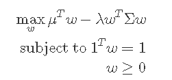
The Markowitz Mean-Variance Portfolio is constructed as follows:
We can set different risk parameters by adjusting and see how the returns are affected. This can be done by running multiple optimisation problems on the data with different values. Higher values places emphasis on the right hand side of the equation and thus the more risk adverse the investor is.
We can see how the risk and return is affected by the changes in the values in the following plot. As the values increase the less risk we take on but also we assume less returns. Low values of makes us invest in a signle asset with the weight on asset , increasing the values increases the weights in other assets spreading our risk.
Note: I originally made this post a few months back and when I went back to it some of the parts for the Max-Sharpe Ratio portfolio did not work as before – I think this is due to the recent update in the tidyr package. I made some minor adjustments, however this part of the post is incorrect (just look at the portfolio weights plot). I hightlight in the code when I made the minor adjustments – when I have the opportunity to go back through the code more carefully I will –
# 2) Function: Max Sharpe Ratio
#NOTE::: When we have all negative mus for a given month we obtain an NA value - the function
# cannot find a maximum when all mus are negative compare the MaxSharpePortfolio$`2015 Sep` and
# MaxSharpePortfolio$`2015 Oct` along with the mus$`2015 Sep` and mus$`2015 Oct` we invests 99% of the portfolio
# in Sept in ABBV since its positive. In Oct ABBV mu is negative and we cannot invest at all.
# Increasing the universe of Assets may overcome this problem.
MaxSharpeportolioFunction <- function(mu, Sigma) {
  w <- Variable(nrow(Sigma))
  problem <- Problem(
    Minimize(quad_form(w, Sigma)),
    constraints = list(
      w >= 0, t(mu) %*% w == 1)
  )
  Solution <- solve(problem, solver="SCS")
  return(as.vector(Solution$getValue(w)/sum(Solution$getValue(w))))
}

# 3a) Portfolio Max Sharpe Ratio
MaxSharpePortfolio <- purrr::map2(.x = mus,
                                  .y = Sigmas,
                                  .f = ~MaxSharpeportolioFunction(.x, .y))

# 3b) Portfolio Max Sharpe Ratio
  MaxSharpePortfolioWeights <- setNames(MaxSharpePortfolio, ListNamesDates) %>%
    as_tibble(.) %>%               # Made an adjustment here
    map(.,  ~setNames(., c(symbols))) %>%
    map_dfr(., ~bind_rows(.), .id = "date") %>%
    mutate(date = as.Date(paste(date, "01"), format = "%Y %b %d"))

MaxSharpePortfolioWeights %>%
  head() %>%
  kable() %>%
  kable_styling(bootstrap_options = c("striped", "hover", "condensed", "responsive"))
date
AAPL
ABBV
A
APD
AA
CF
NVDA
HOG
WMT
AMZN
2013-07-01
0.0009088
0.1532283
0.0371040
0.2332344
-0.1010233
0.0126946
0.2083815
-0.0262255
0.5086221
-0.0269248
2013-08-01
0.0109744
0.1485344
-0.0156878
0.3292178
-0.0080488
0.0051372
0.1146053
0.0091278
0.4086911
-0.0025515
2013-09-01
0.1217206
0.1246626
0.0087004
0.3421645
0.0000000
0.0000000
0.2414533
0.0002820
0.1610166
0.0000000
2013-10-01
0.0270424
0.0000000
0.2268394
0.3427932
0.0000000
0.0000000
0.2653166
0.1283026
0.0000000
0.0097059
2013-11-01
0.2061379
0.0000000
0.1890218
0.2234739
0.0000000
0.0533254
0.0000000
0.0000000
0.0000000
0.3280410
2013-12-01
0.2252115
0.0000000
0.0306323
0.0724210
0.0000000
0.0325004
0.0000000
0.1907158
0.1192395
0.3292796
# 3c) Portfolio Max Sharpe Ratio
MaxSharpePortfolioWeights %>%
  select(date, everything()) %>%      # Made an adjustment here
  pivot_longer(cols = 2:ncol(.), values_to = "weights") %>%
  ggplot(aes(fill = name, y = weights, x = date)) +
  geom_bar(position = "stack", stat = "identity", width = 100) +
  scale_fill_viridis(option = "magma", discrete = TRUE, name = "Asset") +
  theme_bw() +
  ggtitle("Maximum Sharpe Ratio Rolling Portfolio Adjustments") +
  xlab("Date") +
  ylab("Weights")
Looking at the plots the Global Minimum Variance Portfolio shows the lowest volatility in the portfolio returns. The Max Sharpe portfolio is clearly wrong here (see, previous point on Max Sharpe Ratio section). The annaulised performance metrics are also displayed at the bottom for each portfolio over the period.
Plotting the cumulative returns shows that the Markowitz lambda portfolios have the highest returns over the period, however they also have the highest standard deviation over the same period.
chart.CumReturns(AllReturns, main = "Weighted Returns by Objective Function and Risk Tolerance",
                 wealth.index = TRUE, legend.loc = "topleft", colorset = rich6equal)
charts.PerformanceSummary(AllReturns, main = "Performance for Different Weighted Assets",
                          wealth.index = TRUE, colorset = rich6equal)
Additional
(Some additional test data I leave here for future reference)

 is a portfolio of assets with gives us the lowest possible return variance or portfolio volatility. Volatility here is used as a replacement for risk, thus with less variance in volatility correlates to less risk in an asset. The portfolio focuses only on risk and ignores expected returns.
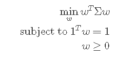
 is unknown we can estimate it as
  with the covariance matrix. In which the convex solution becomes:
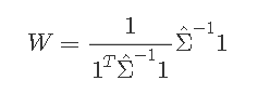
 problem
  . The
. The  where
where  is a vector and
  is a matrix or in our case ww is our weights vector and
  . The
. The  in which we cannot assign negative weights to our assets and that we invest all our capital in the portfolio.
 and see how the returns are affected. This can be done by running multiple optimisation problems on the data with different
  , increasing the
  spreading our risk.


