
Gradient descent is one of the most important ideas in machine learning: given some cost function to minimize, the algorithm iteratively takes steps of the greatest downward slope, theoretically landing in a minima after a sufficient number of iterations. First discovered by Cauchy in 1847 but expanded upon in Haskell Curry for non-linear optimization problems in 1944, gradient descent has been used for all sorts of algorithms, from linear regression to deep neural networks.
While gradient descent and its repurposing in the form of backpropagation has been one of the greatest breakthroughs in machine learning, the optimization of neural networks remain an unsolved problem. Many on the Internet are willing to go as far as to declare that ‘gradient descent sucks’, and while that may be a bit far, it is true that gradient descent has many issues.
- Optimizers get caught up in local minima that are deep enough. Admittedly, there are clever solutions to sometimes get around these issues, like momentum, which can carry optimizers over large hills; stochastic gradient descent; or batch normalization, which smooths the error space. Local minima is still the root cause of many branching problems in neural networks, though.
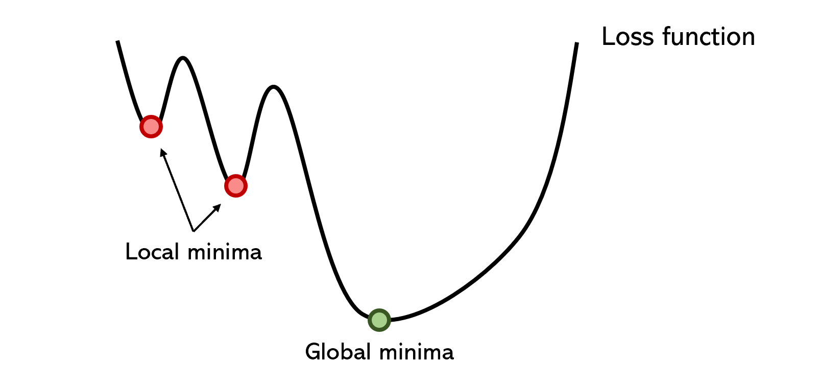
- Because optimizers are so tempted by local minima, even if it manages to get out of it, it takes a really, really long time. Gradient descent is generally a lengthy method because of its slow convergence rate, even with adaptations for large datasets like batch gradient descent.
- Gradient descent is especially sensitive to the initialization of the optimizer. For instance, performance may be much better if the optimizer is initialized near the second local minima instead of the first, but this is all determined randomly.
- Learning rates dictate how confident and risky the optimizer is; setting too high a learning rate may cause it to overlook global minima whereas too low a learning causes the runtime to blow up. To address this problem, learning rates have evolved with decaying, but choosing the rate of decay, among many other variables dictating the learning rate, is difficult.
- Gradient descent requires gradients, meaning that it is prone to gradient-based problems like vanishing or exploding gradient problems, in addition to its inability to handle nondifferentiable functions.
Of course, gradient descent has been extensively studied, and there are many proposed solutions — some which are GD variations and others that are network architecture-based — that work in some cases. Just because gradient descent is overrated doesn’t mean it’s not the best possible solution available currently. Commonplace knowledge like using batch normalization to smooth the error space or picking a sophisticated optimizer like Adam or Adagrad are not the focus of this article, even if they generally perform better.
Instead, the purpose of this writing is to shed some well-deserved light onto more obscure and certainty interesting optimization methods that don’t fit the standard bill of being gradient-based, which, like any other technique used to improve the performance of the neural network, work exceptionally well in some scenarios and not so well in others. Regardless of how well they perform on a specific task, however, they are fascinating, creative, and a promising area of research for the future of machine learning.
Particle Swarm Optimization is a population-based method thatdefines a set of ‘particles’ that explore the search space, attempting to find a minimum. PSO iteratively improved a candidate solution with respect to a certain quality metric. It solves the problem by having a population of potential solutions (‘particles’) and moving them around according to simple mathematical rules like the particle’s position and velocity. Each particle’s movement is influenced by the local position it believes is best, but is also attracted by the best known positions in the search-place (found by other particles). In theory, the swarm moves over several iterations towards the best solutions.
PSO is a fascinating idea — it is much less sensitive to initialization than neural networks, and the communication between particles on certain findings could prove to be a very efficient method of searching sparse and large areas.
Because Particle Swarm Optimization is not gradient-based (gasp!), it does not require the optimization problem to be differentiable; hence using PSO to optimize a neural network or any other algorithm would allow more freedom and less sensitivity on the choice of activation function or equivalent role in other algorithms. Additionally, it makes little to no assumptions about the problem being optimized and can search very large spaces.
As one may imagine, population-based methods can be a fair bit more computationally expensive than gradient-based optimizers, but not necessarily so. Because the algorithm is so open and non-rigid — as evolution-based algorithms often are, one can control the number of particles, the speed at which they move, the amount of information that is shared globally, and so on; just like one might tune learning rates in a neural network.
Surrogate optimization is a method of optimization that attempts to model the loss function with another well-established function to find the minima. The technique samples ‘data points’ from the loss function, meaning it tries different values for parameters (the x) and stores the value of the loss function (the y). After a sufficient number of data points have been collected, a surrogate function (in this case, a 7th-degree polynomial) is fitted to the collected data.
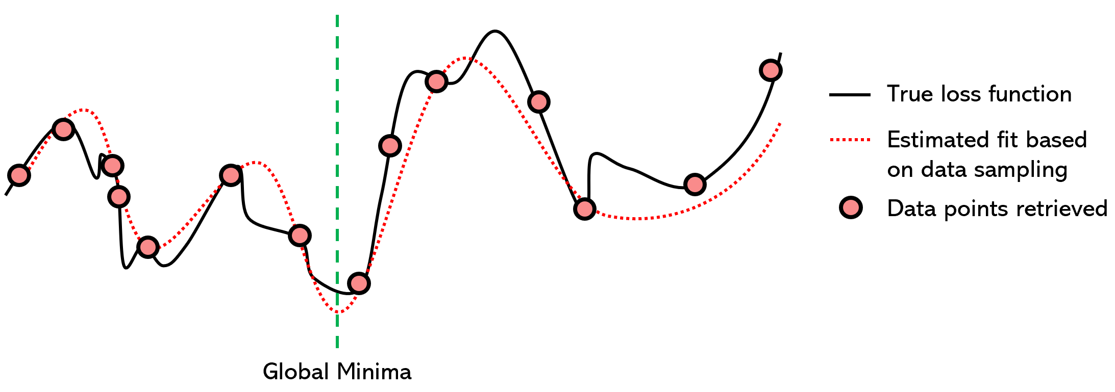
Because finding the minima of polynomials is a very well-studied subject and there exist a host of very efficient methods to find the global minima of a polynomial using derivatives, we can assume that the global minima of the surrogate function is the same for the loss function.
Surrogate optimization is technically a non-iterative method, although the training of the surrogate function is often iterative; additionally, it is technically a no-gradient method, although often effective mathematical methods to find the global minima of the modelling function are based on derivatives. However, because both the iterative and gradient-based properties are ‘secondary’ to surrogate optimization, it can handle large data and non-differentiable optimization problems.
Optimization using a surrogate function is quite clever in a few ways:
- It is essentially smoothing out the surface of the true loss function, which reduces the jagged local minima that cause so much of the extra training time in neural networks.
- It projects a difficult problem into a much easier one: whether it’s a polynomial, RBF, GP, MARS, or another surrogate model, the task of finding the global minima is boosted with mathematical knowledge.
- Overfitting the surrogate model is not really much of an issue, because even with a fair bit of overfitting, the surrogate function is still more smooth and less jagged than the true loss function. Along with many other standard considerations in building more mathematically-inclined models that have been simplified, training surrogate models is hence much easier.
- Surrogate optimization is not limited by the view of where it currently is in that it sees the ‘entire function’, opposed to gradient descent, which must continually make risky choices on whether it thinks there will be a deeper minima over the next hill.
Surrogate optimization is almost always faster than gradient descent methods, but often at the cost of accuracy. Using surrogate optimization may only be able to pinpoint the rough location of a global minima, but this can still be tremendously beneficial.
An alternative is a hybrid model; a surrogate optimization is used to bring the neural network parameters to the rough location, from which gradient descent can be used to find the exact global minima. Another is to use the surrogate model to guide the optimizer’s decisions, since the surrogate function can a) ‘see ahead’ and b) is less sensitive to specific ups and downs of the loss function.
Simulated Annealing is a concept based on annealing in metallurgy, in which a material can be heated above its recrystallization temperature to reduce its hardness and alter other physical and occasionally chemical properties, then allowing the material to gradually cool and become rigid again.
Using the notion of slow cooling, simulated annealing slowly decreases the probability of accepting worse solutions as the solution space is explored. Because accepting worse solutions allows for a more broad search for the global minima (think — cross the hill for a deeper valley), simulated annealing assumes that the possibilities are properly represented and explored in the first iterations. As time progresses, the algorithm moves away from exploration and towards exploitations.
The following is a rough outline of how simulated annealing algorithms work:
- The temperature is set at some initial positive value and progressively approaches zero.
- At each time step, the algorithm randomly chooses a solution close to the current one, measures its quality, and moves to it depending on the current temperature (probability of accepting better or worse solutions).
- Ideally, by the time the temperature reaches zero, the algorithm has converged on a global minima solution.
The simulation can be performed with kinetic equations or with stochastic sampling methods. Simulated Annealing was used to solve the travelling salesman problem, which tries to find the shortest distance between hundreds of locations, represented by data points. Obviously, the combinations are endless, but simulated annealing — with its reminiscence of reinforcement learning — performs very well.

Simulated annealing performs especially well in scenarios where an approximate solution is required in a short period of time, outperforming the slow pace of gradient descent. Like surrogate optimization, it can be used in hybrid with gradient descent for the benefits of both: the speed of simulated annealing and the accuracy of gradient descent.
This was a small sampling of no-gradient methods; there exist many additional algorithms like pattern search and multi-objective optimization to be explored. Genetic and population-based algorithms like particle swarm optimization are extremely promising for creating truly ‘intelligent’ agents, given that we, humans, are evidence of its success.
Non-gradient methods for optimization are fascinating because of the creativity many of them utilize, not being restricted by the mathematical chains of gradients. No one expects no-gradient methods to go mainstream ever because gradient-based optimization performs so well even considering its many problems. However, harnessing the power of no-gradient and gradient-based methods with hybrid optimizers demonstrates extremely high potential, especially in an era where we are reaching a computational limit.
