
In this article, I cover the terminology needed to get acquainted with genetic algorithms, walk through an example where we would like a high-precision estimator of the optima for a single-objective optimization problem, then discuss the importance of parameter tuning and the forces that drive the evolution of a genetic algorithm’s population.
Genetic Algorithms
Genetic Algorithms (GAs) are meta-heuristic algorithms inspired by Darwin’s theory of natural selection and that belong to a broader class of evolutionary algorithms (EA). In the context of optimization, this principle is used to find good decision variable choices without exhaustively searching the variable space.
Traditionally, genetic algorithms are known to be difficult to use for solving high-precision estimators of optima in single-objective optimization problems. In the case of smooth continuous functions, GAs are outclassed by algorithms like the canonical Newton’s method. Nonetheless, our demonstration will make use of a simple GA on a simple smooth function.
Terminology
Before we begin, it is important to lay the foundation with a firm understanding of the terminology used when developing a genetic algorithm for a problem that we are working on. Let us consider the following problem:
Let’s plot the function to see what we are working with.
import matplotlib.pyplot as plt
def f(x):
    return (x*np.sin(6*pi*x)) #Function being optimized
x = np.arange(-0.75, 1.3, 0.01)
y = f(x)
plt.plot(x,y)
plt.xlabel('Value of x')
plt.ylabel('Value of Function')
plt.title('Objective Function')
plt.legend()
plt.show()
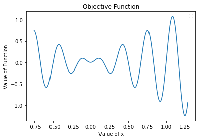
The decision variable x will be represented by a vector of length 6, where the first element is a real number in [-1, 1] and the remaining elements are integers in [0, 9]. The first element will determine the sign of , x. That is, if the first element is greater than or equal to 0, we will have a positive value of x, otherwise it is negative. For example, the candidate solution x = (-0.5423, 1, 1, 5, 4, 9) represents x = –1.1549.
Now, let’s walk through each term that helps us describe the problem in the context of genetic algorithms.
Gene
A gene is a decision variable. In our problem, x is represented by a vector of 6 elements, each of which we will be choosing a value for. Thus, each of these elements is a gene.
Chromosome
The chromosome is a vector of a problem’s genes. Thus, the vector representing x is our chromosome.
Genotype
A genotype is a combination of all decision variables relevant to a problem, forming a candidate solution to the optimization problem. Thus, a particular combination of values for each gene in our chromosome, say x = (0.3455, 3, 6, 1, 5, 8) is a genotype.
Phenotype
A phenotype is a combination of all of the optimization criteria relevant to a problem. Since in this problem we are optimizing for only one function, f, this represents our only phenotype.
Character
A character is one of potentially many optimization criteria relevant to a problem. Again, since we are working with only one function, f, this is our only character.
Trait
A trait is the evaluated value of one of the optimization criteria for a given genotype. For our problem, consider again the genotype x = (0.3455, 3, 6, 1, 5, 8). This corresponds to x = 3.6158. Then f(3.6158)= -2.9696 is the trait of this particular genotype.
Fitness
The fitness of a solution gives us an idea of how good a genotype is at solving out problem. In our example, since we are maximizing a function, a larger value trait for a genotype corresponds to a better fitness.
Parent
At any stage of the algorithm, we will have a population of candidate solutions. In each iteration, or generation, of the algorithm, some candidate solutions we be selected to survive into the next generation and to produce some children.
Children
New candidate solutions produced by selected parents from the previous generation.
Now, we can confidently proceed to the algorithm.
The Algorithm
Full code can be found here: https://github.com/guerreropeinado/GABase10-Genotype/blob/master/TD_GA.py
The algorithm we will demonstrate can be defined compactly:
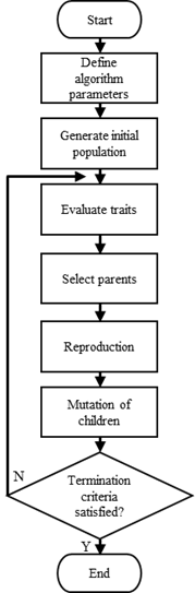
The algorithm parameters we begin with are the number of candidate solutions in the population at the start of each generation and the number of generations to run the algorithm, which also serves as our stopping condition.
Now, we’ll walk through each step of the algorithm. First, let’s import each of our libraries used:
import numpy as np
from math import  pi
Initial Population
For a given choice of population size, we generate an initial population of genotypes. There are different ways one can do this, here we generate each gene of each candidate solution randomly.
The code for this is shown here:
def initialize_population(population_size):
    '''
    Initialize a population randomly

    Arguments:
    population_size -- even integer that represents the number of candidate solutions considered in each generation

    Returns
    population -- Collection of candidate solutions, each represented by an array where each element represents a digit of the solution
    '''
    population = []
    for j in range(population_size):
        x1 = np.random.uniform(low =-1, high =1) #Value that will determine the sign of the candidate solution
        x2 = np.random.randint(low=0, high=9, size = 5)
        x = np.append(x1,x2)
        population = np.append(population,x)
    population = np.split(population, population_size)
    return population
Fitness Evaluation
With a population in hand, we can now begin the algorithm by evaluating the trait of each candidate solution.
Notice that for certain values of x, we assign a low value of fitness. We do this for values of x that violate the constraints of our optimization problem. This will make it so that infeasible solutions are less likely to survive into the next generation. We are careful to not set this fitness value too low, as these infeasible solutions may still contain some values in their genotype that may be useful for advancing the population towards good solutions.
def evaluate_fitness(pop):
    '''
    Evaluates the fitness of each candidate solution in the population

    Arguments:
    pop -- the current set of candidate solutions

    Returns
    fitness -- an array with the fitness evaluated for each candidate solution
    '''
    population_size = len(pop)
    fitness = []
    for j in range(population_size):
        ind = pop[j]
        if ind[0]>=0:
            sign = 1
        else:
            sign = -1
        x = sign*float(str((int(ind[1])))+"."+str((int(ind[2])))+str((int(ind[3])))+str((int(ind[4])))+str((int(ind[5]))))
        if x<-0.75 or x>1.3: #Solutions that violate the constraints will be penalized with low fitness value
            fit = -1
        else:
            fit = f(x)
        fitness = np.append(fitness,fit)
    return fitness
Selection
We now have a population and a value of fitness (trait) for each candidate solution. There are various methods for selecting parents from the given population. Here we will use the canonical method of tournament selection.
With tournament selection, we sample, with replacement, m candidate solutions from the population. The candidate solution with the best value of fitness is added to the parent pool and will survive into the next generation and have the chance to produce children. This is performed n times.
Choices of m and n can be adjusted by the modeler. Here we are implicitly using m=2 and taking n as user input.
def tournament_selection(population, fitness, num_parents):
    '''
    Performs tournament selection to select solutions that will make it to the next generation and
    will be given the chance to produce offspring

    Arguments:
    population -- the current set of candidate solutions
    fitness -- evaluated fitness for each candidate solution in the current population
    num_parents -- the number of head-to-head tournaments

    Returns
    parents -- a set of candidate solutions that will be used in the next generation and may produce offspring
    '''
    parents =[]
    for i in range(num_parents):
        index1 = np.random.randint(low=0, high=num_parents-1)
        index2 = np.random.randint(low=0, high=num_parents-1)
        #Choose which individual becomes a parent
        if fitness[index1] > fitness[index2]:
            parents = np.append(parents, population[index1])
        else:
            parents = np.append(parents, population[index2])
    parents = np.split(parents, num_parents)
    return parents
Reproduction
With our population down to the number of selected parents, we need reproduction to get our population back to its original size. Like with selection, there are many methods to perform reproduction. Here we will be showcasing single-point crossover.
Single-point cross over is performed by taking a portion of one parent, the remaining portion of another parent, and combining them to form a child. Here we will do this by sampling, with replacement, to candidate solutions form the parents, taking the first 2 elements of the first parent, the last 4 elements of the second parent, then combining. This is illustrated below:

def single_point_crossover(parents, num_offspring):
    '''
    Samples, with replacement, from parents and performs single-point crossover to produce offspring for next generation

    Arguments:
    parents -- a set of candidate solutions that will be used in the next generation and may produce offspring
    num_offspring -- the number of offspring to produce

    Returns
    children -- a set of candidate solutions that will be used in the next generation
    '''
    children = []
    for i in range(num_offspring):
        index1 = np.random.randint(low=0, high=9)
        index2 = np.random.randint(low=0, high=9)
        parent1 = parents[index1]
        parent2 = parents[index2]
        offspring = np.append(parent1[0:2],parent2[2:6])
        children = np.append(children, offspring)
    children = np.split(children, num_offspring)
    return children
Mutation
With mutation, we seek to add some diversity to our population in hopes that it will pave the way for unearthing some new good solutions. Here we perform mutation on the set of children by, for each gene of each candidate solution, drawing a random uniform number in [0, 1]. If this number is below some threshold, we change the value of the gene to a random integer in [0, 9].
def mutation(children):
    '''
    Randomly adjust some genotypes of some of the offspring produced for the next generation

    Arguments:
    children -- a set of candidate solutions that will be used in the next generation

    Returns
    children -- a set of candidate solutions that will be used in the next generation
    '''
    num_offspring = len(children)
    for i in range(num_offspring):
        for j in range(1,6):
            prob = np.random.uniform(low=0, high=1)
            if prob < 0.5:
                random_value = np.random.randint(low=0, high=9)
                children[i][j] = random_value
    return children
All Together
Using the above components, we place it all together in order to run a fully functional genetic algorithm. Note that we set the termination condition as the number of generations to run the algorithm, however, as the population may converge sooner it would be good to place a stop check on this event.
def genetic_algorithm(num_generations, population_size):
    '''
    Perform the genetic algorithm

    Arguments:
    num_generations -- the number of iterations to perform the algorithm
    population_size -- even integer that represents the number of candidate solutions considered in each generation

    Returns:
    best_OF_value -- the best value of the objective function found by the algorithm
    best_solution -- the candidate solutions giving the best value of the objective function found by the algorithm
    '''
    population = initialize_population(population_size)
    for gen in range(num_generations):
        fitness = evaluate_fitness(population)
        parents = tournament_selection(population,fitness,num_parents =int(population_size/2))
        children = single_point_crossover(parents, num_offspring = int(population_size/2))
        children = mutation(children)
        population  = np.append(parents,children)
        population = np.split(population, population_size)
    fitness = evaluate_fitness(population)
    best_solution_index = np.argmax(fitness)
    best_OF_value = max(fitness)
    ind = population[best_solution_index]
    if ind[0]>=0:
        sign = 1
    else:
        sign = -1
    best_solution = sign*float(str((int(ind[1])))+"."+str((int(ind[2])))+str((int(ind[3])))+str((int(ind[4])))+str((int(ind[5]))))
    return best_OF_value, best_solution
Trial Run
Let’s try our developed algorithm with 100 generations and a population size of 100 on our problem:
best_OF_value, best_solution = genetic_algorithm(num_generations = 100, population_size=100)
print("The largest value of the objective function is: ",  best_OF_value)
print("The corresponding solution is x = ",  best_solution)
The output is
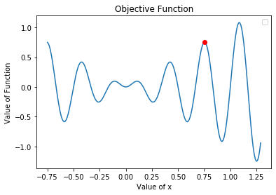
The largest value of the objective function is:  1.0842377727119092
The corresponding solution is x =  1.0845
Note that this solution was from a single run. A different solution can be found on a different run considering that our population is initiated randomly and can evolve in different directions. Let’s plot this solution along with our objective function
x = np.arange(-0.75, 1.3, 0.01)
y = f(x)
plt.plot(x,y)
plt.plot(best_solution,best_OF_value,'ro')
plt.xlabel('Value of x')
plt.ylabel('Value of Function')
plt.title('Objective Function')
plt.legend()
plt.show()
Our algorithm has converged at a local optimum on this run. To gain some insight on how our choices of population size and number of generations effects the results, let’s run the same instance of the algorithm 100 times and plot the average solution found.
Average = 0
for i in range(0,100):
    best_OF_value, best_solution = genetic_algorithm(num_generations = 100, population_size=100)
    Average+=best_solution
Average = Average/100
z = f(Average)x = np.arange(-0.75, 1.3, 0.01)
y = f(x)
plt.plot(x,y)
plt.plot(Average,z,'ro')
plt.xlabel('Value of x')
plt.ylabel('Value of Function')
plt.title('Objective Function')
plt.legend()
plt.show()

As it turns out, the solution we found on out first run was much better than what our algorithm would find in most searches. Let’s plot the same average algorithm result again, but this time using a population size of 1,000! This will take a while to run on even the most up-to-date consumer processors.

Now even on average, the algorithm is able to come close to the true optimal solution. This demonstrates the importance of parameter selections. Next, we’ll discuss more about this and provide some intuition on what drives the population’s movement through our variable space.
Parameter Tuning
Most algorithms you will encounter will need to have some parameters tuned in order to perform well on their assigned task. Genetic algorithms are no exception.
We often encounter the phrase, “exploration vs exploitation”. In optimization, this refers to the trade-off between having the algorithm explore new areas of the search space and using already detected points to search for the optimum. Parameter selection is crucial in striking a good balance between these objectives.
In genetic algorithms, as our population evolves from generation to generation it is subject to forces that determine the trade-off being made between exploration vs exploitation. Namely, there are three forces to be aware of:
- Drift Force: Genetic drift is the change in the frequency of an existing value for a gene. What this force does is cause the individuals in a population to become more and more similar, until the population has converged.
- Selection Force: There is pressure on the population to find good solutions to the problem. This means that good solutions continue to pass on all/some of their genes until it is widespread in the population. Hence, this force also drives the population towards convergence.
- Mutation Force: The way we can combat selection and drift pressure in order to avoid premature population convergence is through mutation. Mutation allows us to add diversity into the population so that more exploration can be done before the population converges.
Designing genetic algorithms that do well in balancing exploration and exploitation is still a very active area of research. However, there are a couple of things you can keep in mind when tailoring them to your problems:
- Mutation can balance drift at the cost of limiting selection
- Drift has a smaller effect on larger populations
- At the cost of algorithm speed, you can increase population size to increase precision
- For accuracy, start and maintain a diverse population in order to provide exploration pressure
The reader is encouraged to play with the various parameters (mutation rate, population size, and even changing the selection and reproduction methods) in order to see each of the discussed forces at work.
