
From: https://towardsdatascience.com/cluster-then-predict-for-classification-tasks-142fdfdc87d6

Introduction
Supervised classification problems require a dataset with (a) a categorical dependent variable (the “target variable”) and (b) a set of independent variables (“features”) which may (or may not!) be useful in predicting the class. The modeling task is to learn a function mapping features and their values to a target class. An example of this is Logistic Regression.
Unsupervised learning takes a dataset with no labels and attempts to find some latent structure within the data. K-means is one such algorithm. In this article, I will show you how to increase your classifier’s performance by using k-means to discover latent “clusters” in your dataset and either use these clusters as new features in your dataset or to partition your dataset by cluster and train a separate classifier on each.
Dataset
We begin by generating a nonce dataset using sklearn’s make_classification utility. We will simulate a multi-class classification problem and generate 15 features for prediction.
from sklearn.datasets import make_classificationX, y = make_classification(n_samples=1000, n_features=8, n_informative=5, n_classes=4)
We now have a dataset of 1000 rows with 4 classes and 8 features, 5 of which are informative (the other 3 being random noise). We convert these to a pandas dataframe for easier manipulation.
import pandas as pddf = pd.DataFrame(X, columns=['f{}'.format(i) for i in range(8)])
Divide into Train/Test
We can now divide our data into a train and test set (75/25) split.
from sklearn.model_selection import train_test_splitX_train, X_test, y_train, y_test = train_test_split(df, y, test_size=0.25, random_state=90210)
Applying K-means
Firstly, you will want to determine what the optimal k is given the dataset.
For the sake of brevity and so as not to distract from the purpose of this article, I refer the reader to this excellent tutorial: How to Determine the Optimal K for K-Means? should you want to read further on this matter.
In our case, because we used the make_classification utility, the parameter
n_clusters_per_class
is already set and defaults to 2. Therefore, we do not need to determine the optimal k; however, we do need to identify the clusters! We will use the following function to find the 2 clusters in the training set, then predict them for our test set.
import numpy as np
from sklearn.cluster import KMeans
from typing import Tupledef get_clusters(X_train: pd.DataFrame, X_test: pd.DataFrame, n_clusters: int) -> Tuple[pd.DataFrame, pd.DataFrame]:
    """
    applies k-means clustering to training data to find clusters and predicts them for the test set
    """
    clustering = KMeans(n_clusters=n_clusters, random_state=8675309,n_jobs=-1)
    clustering.fit(X_train)
    # apply the labels
    train_labels = clustering.labels_
    X_train_clstrs = X_train.copy()
    X_train_clstrs['clusters'] = train_labels

    # predict labels on the test set
    test_labels = clustering.predict(X_test)
    X_test_clstrs = X_test.copy()
    X_test_clstrs['clusters'] = test_labels
    return X_train_clstrs, X_test_clstrsX_train_clstrs, X_test_clstrs = get_clusters(X_train, X_test, 2)
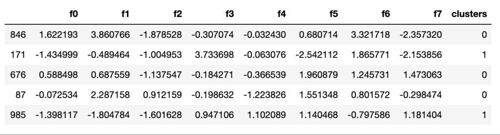
We now have a new feature called “clusters” with a value of 0 or 1.

Scaling
Before we fit any models, we need to scale our features: this ensures all features are on the same numerical scale. With a linear model like logistic regression, the magnitude of the coefficients learned during training will depend on the scale of the features. If you had features that were on the scale of 0–1 and other features on the scale of say 0–100, the coefficients could not be reliably compared.
To scale the features, we use the following function which computes z-scores for each of the features and maps the learnings from the train set to the test set.
from sklearn.preprocessing import StandardScalerdef scale_features(X_train: pd.DataFrame, X_test: pd.DataFrame) -> Tuple[pd.DataFrame, pd.DataFrame]:
    """
    applies standard scaler (z-scores) to training data and predicts z-scores for the test set
    """
    scaler = StandardScaler()
    to_scale = [col for col in X_train.columns.values]
    scaler.fit(X_train[to_scale])
    X_train[to_scale] = scaler.transform(X_train[to_scale])

    # predict z-scores on the test set
    X_test[to_scale] = scaler.transform(X_test[to_scale])

    return X_train, X_testX_train_scaled, X_test_scaled = scale_features(X_train_clstrs, X_test_clstrs)
We are now ready to run some experiments!
Experimentation
I chose to use Logistic Regression for this problem because it is extremely fast and inspection of the coefficients allows one to quickly assess feature importance.
To run our experiments, we will build a logistic regression model on 4 datasets:
- Dataset with no clustering information(base)
- Dataset with “clusters” as a feature (cluster-feature)
- Dataset for df[“clusters”] == 0 (clusters-0)
- Dataset for df[“clusters”] == 1 (clusters-1)
Out study is a 1×4 between-groups design with dataset [base, cluster-feature, clusters-0, clusters-1] as the only factor. The following creates our datasets.
# to divide the df by cluster, we need to ensure we use the correct class labels, we'll use pandas to do that
train_clusters = X_train_scaled.copy()
test_clusters = X_test_scaled.copy()
train_clusters['y'] = y_train
test_clusters['y'] = y_test# locate the "0" cluster
train_0 = train_clusters.loc[train_clusters.clusters < 0] # after scaling, 0 went negtive
test_0 = test_clusters.loc[test_clusters.clusters < 0]
y_train_0 = train_0.y.values
y_test_0 = test_0.y.values# locate the "1" cluster
train_1 = train_clusters.loc[train_clusters.clusters > 0] # after scaling, 1 dropped slightly
test_1 = test_clusters.loc[test_clusters.clusters > 0]
y_train_1 = train_1.y.values
y_test_1 = test_1.y.values# the base dataset has no "clusters" feature
X_train_base = X_train_scaled.drop(columns=['clusters'])
X_test_base = X_test_scaled.drop(columns=['clusters'])# drop the targets from the training set
X_train_0 = train_0.drop(columns=['y'])
X_test_0 = test_0.drop(columns=['y'])
X_train_1 = train_1.drop(columns=['y'])
X_test_1 = test_1.drop(columns=['y'])datasets = {
    'base': (X_train_base, y_train, X_test_base, y_test),
    'cluster-feature': (X_train_scaled, y_train, X_test_scaled, y_test),
    'cluster-0': (X_train_0, y_train_0, X_test_0, y_test_0),
    'cluster-1': (X_train_1, y_train_1, X_test_1, y_test_1),
}


To efficiently run our experiments, we’ll use the following function which loops through the 4 datasets and runs 5-fold cross-valdiation on each. For each dataset, we obtain 5 estimates for each classifier’s: accuracy, weighted precision, weighted recall, and weighted f1. We will plot these to observe general performance. We then obtain classification reports from each model on its respective test set to evaluate fine-grained performance.
from sklearn.linear_model import LogisticRegression
from sklearn import model_selection
from sklearn.metrics import classification_reportdef run_exps(datasets: dict) -> pd.DataFrame:
    '''
    runs experiments on a dict of datasets
    '''
    # initialize a logistic regression classifier
    model = LogisticRegression(class_weight='balanced', solver='lbfgs', random_state=999, max_iter=250)

    dfs = []
    results = []
    conditions = []
    scoring = ['accuracy','precision_weighted','recall_weighted','f1_weighted']for condition, splits in datasets.items():
        X_train = splits[0]
        y_train = splits[1]
        X_test = splits[2]
        y_test = splits[3]

        kfold = model_selection.KFold(n_splits=5, shuffle=True, random_state=90210)
        cv_results = model_selection.cross_validate(model, X_train, y_train, cv=kfold, scoring=scoring)
        clf = model.fit(X_train, y_train)
        y_pred = clf.predict(X_test)
        print(condition)
        print(classification_report(y_test, y_pred))results.append(cv_results)
        conditions.append(condition)this_df = pd.DataFrame(cv_results)
        this_df['condition'] = condition
        dfs.append(this_df)final = pd.concat(dfs, ignore_index=True)

    # We have wide format data, lets use pd.melt to fix this
    results_long = pd.melt(final,id_vars=['condition'],var_name='metrics', value_name='values')

    # fit time metrics, we don't need these
    time_metrics = ['fit_time','score_time']
    results = results_long[~results_long['metrics'].isin(time_metrics)] # get df without fit data
    results = results.sort_values(by='values')

    return resultsdf = run_exps(datasets)

Results
Let’s plot our results and see how each dataset affected classifier performance.
import matplotlib
import matplotlib.pyplot as plt
import seaborn as snsplt.figure(figsize=(20, 12))
sns.set(font_scale=2.5)
g = sns.boxplot(x="condition", y="values", hue="metrics", data=df, palette="Set3")
plt.legend(bbox_to_anchor=(1.05, 1), loc=2, borderaxespad=0.)
plt.title('Comparison of Dataset by Classification Metric')

pd.pivot_table(df, index='condition',columns=['metrics'],values=['values'], aggfunc='mean')

In general, it appears that our “base” dataset, with no clustering information, creates the worst performing classifier. By adding our binary “clusters” as a feature, we see a modest boost to performance; however, when we fit a model on each cluster, we see the largest boost in performance.
When we look at classification reports for fine-grained performance evaluation, the picture becomes very clear: when the datasets are segmented by cluster, we see a large boost to performance.
base
              precision    recall  f1-score   support

           0       0.48      0.31      0.38        64
           1       0.59      0.59      0.59        71
           2       0.42      0.66      0.51        50
           3       0.59      0.52      0.55        65

    accuracy                           0.52       250
   macro avg       0.52      0.52      0.51       250
weighted avg       0.53      0.52      0.51       250

cluster-feature
              precision    recall  f1-score   support

           0       0.43      0.36      0.39        64
           1       0.59      0.62      0.60        71
           2       0.40      0.56      0.47        50
           3       0.57      0.45      0.50        65

    accuracy                           0.50       250
   macro avg       0.50      0.50      0.49       250
weighted avg       0.50      0.50      0.49       250

cluster-0
              precision    recall  f1-score   support

           0       0.57      0.41      0.48        29
           1       0.68      0.87      0.76        30
           2       0.39      0.45      0.42        20
           3       0.73      0.66      0.69        29

    accuracy                           0.61       108
   macro avg       0.59      0.60      0.59       108
weighted avg       0.61      0.61      0.60       108

cluster-1
              precision    recall  f1-score   support

           0       0.41      0.34      0.38        35
           1       0.54      0.46      0.50        41
           2       0.49      0.70      0.58        30
           3       0.60      0.58      0.59        36

    accuracy                           0.51       142
   macro avg       0.51      0.52      0.51       142
weighted avg       0.51      0.51      0.51       142
Consider the class “0”, the f1 scores across the four datasets are
- Base — “0” F1: 0.38
- Cluster-feature — “0” F1: 0.39
- Cluster-0 — “0” F1: 0.48
- Cluster-1 — “0” F1:0.38
For the “0” class, the model trained on the cluster-0 dataset shows ~23% relative improvement in f1 score over the other models and datasets.
Conclusion and Next Steps
In this article, I have shown how you can leverage “cluster-then-predict” for your classification problems and have teased some results suggesting that this technique can boost performance. There is still much more that can be done in terms of cluster creation and evaluation of the results.
In our case, we had a dataset with 2 clusters; however, in your problems you may have many more clusters to find. (Once you determine the optimal k using the elbow method on your dataset!)
In the case of k>2, you can treat the “clusters” feature as a categorical variable and apply one-hot encoding to use them in your model. As k increases, you may run into issues of overfitting should you decide to fit a model for each cluster. As with all data science problems, experiment, experiment, experiment! Run tests for different techniques and let the data guide your modeling decisions.
