

This work seeks to make Beck et. al, 2018 understandable and put their solutions in a strong background to prepare for understanding of Stochastic Differential Equations.
What are Stochastic Differential Equations?
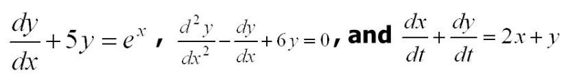
You’ve seen Ordinary Differential Equations.
They are not spooky! They look like so:

What defines an ordinary differential equation is that it is a differential equation containing ONE independent variable with derivatives.
Pulling your math friend, she suggests that these are the following examples of ODEs you can see:
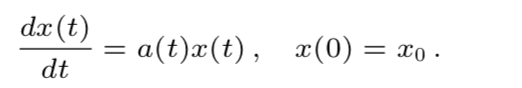
Sometimes you get your math friend to give you the initial conditions,

So we can re-arrange Equation 1 to become the following:
And this is our solution.
Example:
Let’s look at this ODE with the following initial conditions:
Let’s assume that a(t) is not a deterministic parameter [i.e. follows a stochastic parameter]. This stochastic parameter has a drift component that modifies a function where ξ(t) is a white noise process.

Equation 2 thus becomes:

dW(t) is the differential form of the Brownian motion inherent to the stochastic process.
Thus, a Stochastic Differential Equation is:

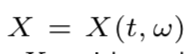
Where w denotes that X = X(t,w) is a Random Variable and possess the initial condition X(0, w) = X_o with probability one.
f (t, X(t,w)), g(t, X(t,w)), W(t,w) is an element of the real space.
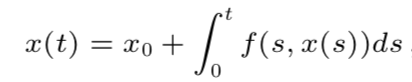
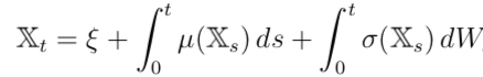
Rewriting Equation 3 into an integral equation we receive:

SDE’s and Kolmogorov Partial Differential “can typically not be solved explicitly”. This is why an approximation is quite helpful.
As seen throughout ESE 303, there are drawbacks on the different ways to generate a numerical methods to an equation. Perhaps it is speed of the operation. Perhaps it is dimensionality.
What if we could use deep learning to approximate a numerical method.
Describing the approximation problem we seek to solve
We are used to partial differential equations such as
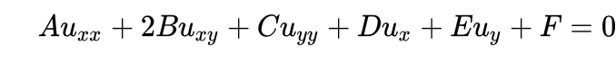
If the coefficients satisfy:
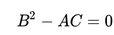
Then it is considered a parabolic partial differential equation.
Given a parabolic partial differential equation:

with initial conditions:

Linearity allows for solutions to be approximated with Monte Carlo simulations at higher dimensions of the problem.
Non-linearity occurs when constraints or frictions are accounted for at similar higher dimensions of the problem.
The goal is to approximate the function p(x,T) on some space R^d.
Derive the approximation problem we seek to solve
Finding u(T,x):
Using the Feynman-Kac formula for the PDE above, Beck et al. adjusted the equation to a PDE using the Feynman-Kac formula (Feynman-Kac formula adapts PDEs to probabilistic & stochastic settings).
They found that the PDE has a u(T,x) of:

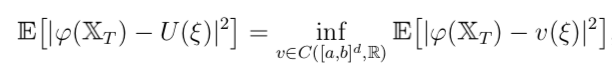
Formulizing as minimisation problem
We seek to turn the above equation into a minimization to approach a solution.
If the above equation 4 can be shown as follpws:
i) The function is twice continuously differentiable with at most polynomially growing derivatives
ii) There is a unique continuous function U such that
iii) U(x) = u(T,x) for every x in the region a to b in dimension d.
Thus we can minimize the expectation value on the right hand side and this is a minimization problem.
Deep Artificial Neural Network Approximations
Of Equation 4, we can make an approximation where

This lets us choose a function U as a deep nearul network.
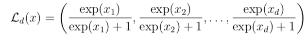
Choosing Ld(x) as a version of the logistic function (activation function) throughout neural networks,

We can make a multidimensional variant of this by setting:
We can create a function which satisfies for every x = (x1, …, xk) be an element of the real space. This is is in essence a larger propagation of the representation across a change of basis from the k basis to the l basis.
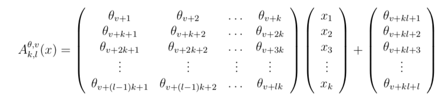
We can derive a function U which satisfies for every theta and x value, the following:

This is in essence the function to be minimized.
Specify the approximation problem we seek to solve
Examples: Heat Equation
Solving the heat equation is trivial with regards to separation of variables.
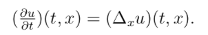
Here is the heat equation, which describes the heat diffusion across space and time along a one dimensional area.
We can receive the following function after solving for u(t,x )

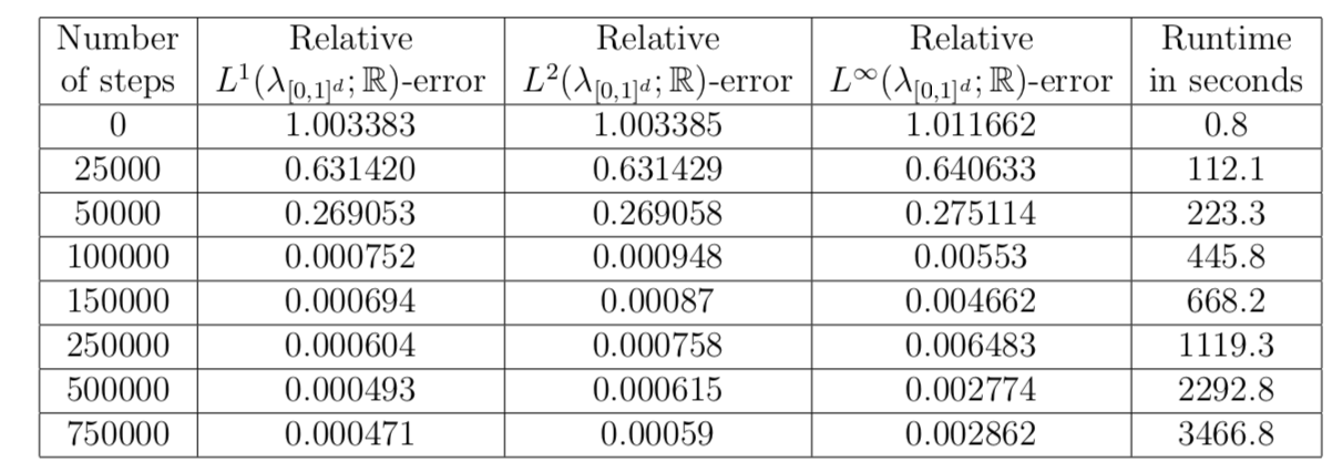
The relative approximation error for L1 is as follows;

The relative approximation error for L2 is as follows:

The relative approximation for long run L at infinity is:

Running the code shows the relative apprioxmation errors
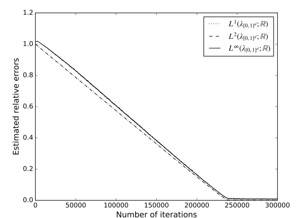
This table shows the relative approximtion errors:

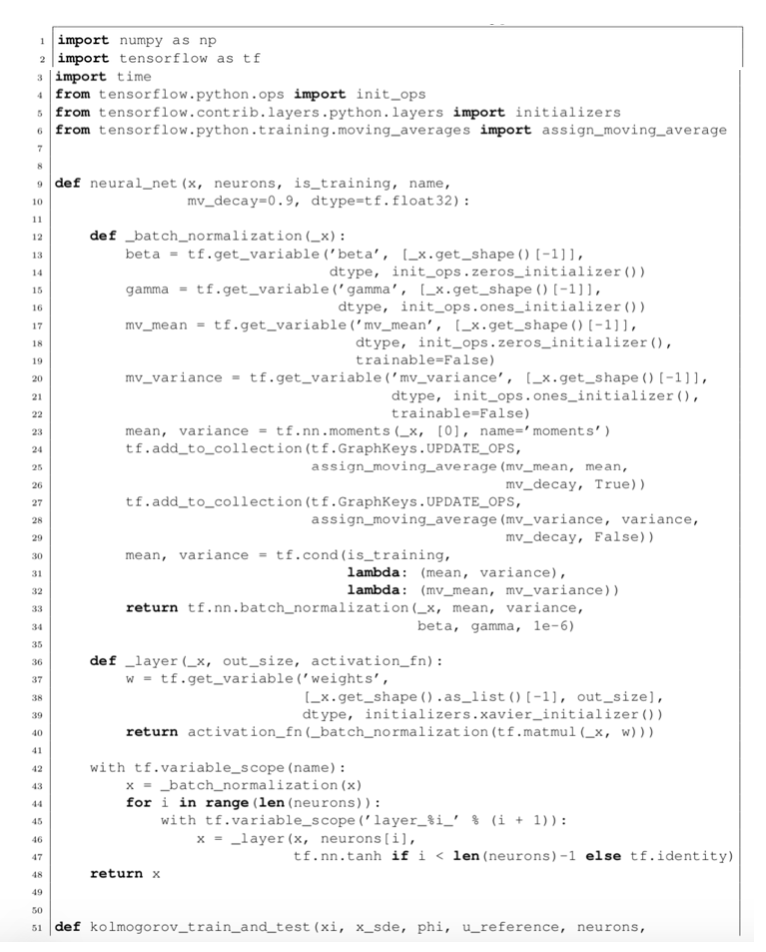
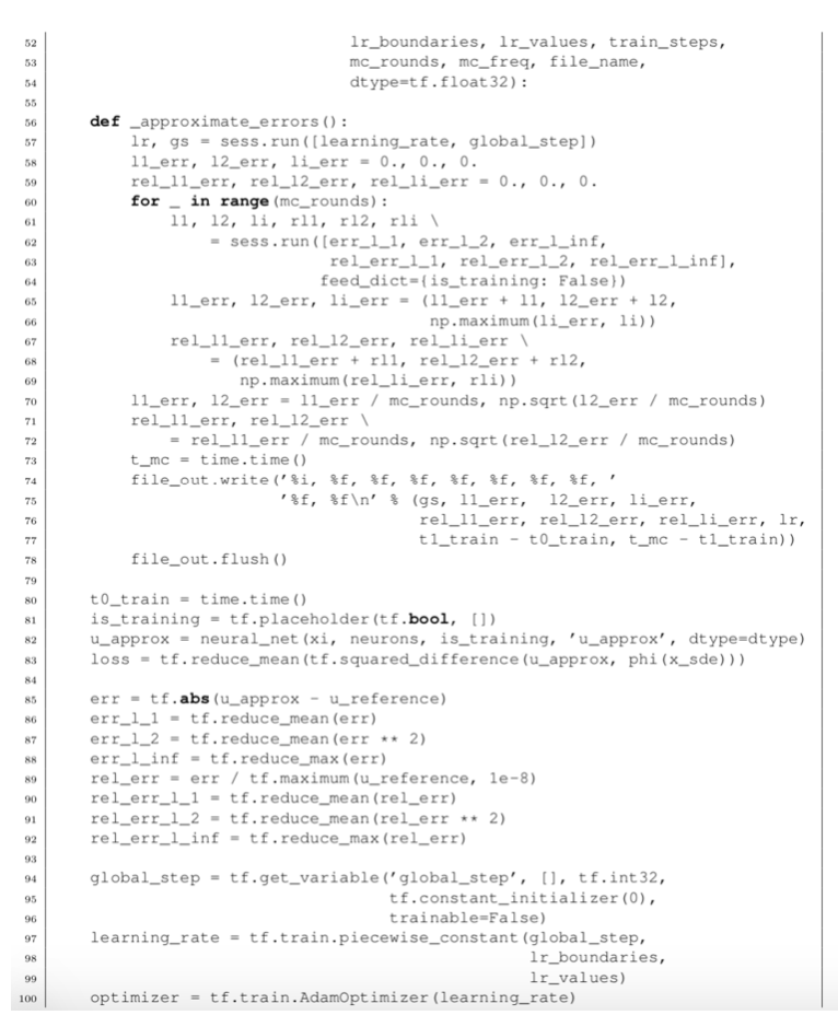
Associated to this is the code:

And here is the python code for the algorithm

This code could also be applied to solve a Black Scholes model.

Where

In essence, there is a way to find a numeric approximation possible for stochsatic differential equations and partial differential equations.
This blog post does not claim credit for the work presented in Beck 2018 but seeks to understand how to make such a numeric approximation possible. These foundations will be layered over in future analyses.
Sources considered:
